Technology for optimization of production of innovative products for civil purpose by enterprises of the Russian defense industrial complex

For multi-product enterprises of the Russian defense industry, the results of modeling intra-company management decisions at the levels of strategic and current production management can be used as a theoretical basis for the technology for optimizing the production of innovative civilian products. They are presented in detail in the works of Danilin V.I., Zhdanov D.A., Pleschinsky A.S. and Stavchikov A.I. [1-5]. Taking into account the industry-specific characteristics of enterprises’ activities in relation to the functional purpose of the tools for modeling innovative activity presented in the above-mentioned works allows for its system optimization, proposed by G.B. Kleiner [6].

Materials and methods

As a modeling object, the activities of a defense industry enterprise with production processes of multi-product innovative products for civilian use, consisting of parallel-sequential stages, will be studied. In the course of their production activities, defense industry enterprises are increasing the production of innovative products in stages. In the future, it is expected to be sold in various markets. A fragment of the network model of the processes occurring in this case is presented in the figure below.

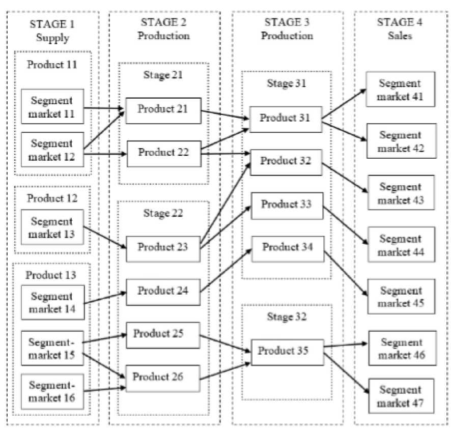
Pic. Network model of production processes and sales of products.

At each stage of production, a certain range of products is produced. It is intermediate and is used at subsequent stages of production. Some of these products are purchased from external suppliers. As a rule, these are initial components for the production of various types of final products. Multiproduct enterprises DIC carry out their activities focusing on various segments of commodity markets. They differ in prices, levels of supply and demand, and volumes of transactions for the purchase of initial and sale of final innovative products for civilian use. The production process is carried out according to the technology used by the enterprise in a specific period of time. It is characterized by the consumption of a certain set of labor resources and equipment to produce a unit of one or another type of innovative product. The consumption of initial and intermediate resources and components for the production of final products is determined by their need. It affects inventory levels at the end of each reporting time period.

The development of a DIC enterprise occurs either as a result of an increase in the volume of resources that are used with the current technology, or through the introduction of a new technology and a corresponding set of production factors in order to produce a modified range of products that meet the new conditions of the markets for innovative products. New, more efficient technology may be purchased from the market or be the result of in-house development. This side of the activity of the DIC enterprise corresponds to the investment or innovation orientation.

When introducing a new technology, it is necessary to take into account the structure of labor resources and the composition of fixed assets, unit costs for the production of innovative products, the level of supply and demand in various segments of product markets, price changes, life cycles of manufactured products, a reduction in the labor intensity of its production due to experience, a new structure of factors production for different periods of time as a result of optimizing the production of innovative products.

The life cycles of manufactured products are taken into account by the permissible change in the minimum and maximum volumes of its production. The manifestation of the experience effect can be determined by a decrease in the labor intensity of production over time. Changes in supply and demand are characterized by the dynamics of price indices in the markets. This side of the DIC enterprise activities corresponds to the operational focus. Attraction of investments occurs as a result of the financial activities of the DIC enterprise, which is designed to ensure its production activities at all stages and time periods with the necessary and sufficient amount of financial resources.

Results and discussion

Optimizing the production of innovative products by DIC enterprises requires increasing their volumes, stocks of initial and intermediate components, reducing possible downtime or additional operating time of labor resources and equipment in various time periods of the enterprise’s operation, developing plans for the supply of initial products and components, as well as the sale of finished products. products in various market segments.

Optimization of the production of innovative products by DIC enterprises is based on the use of an adaptive model. It takes into account a wide range of characteristics of problem situations that arise in practice. Adaptation of the model to the conditions of a specific optimized situation is carried out using a system of parameters. Modeling is performed in the format of an optimization problem of the following type:

A(p a )x = B ,

max F ( x )= c(p c )x + FC ,

a(p b )d).

Here: F ( x ) – criterion, x – vector of required variables, c(p c ) – vector of coefficients c j ( p cj ) of the objective function, FC – fixed value independent of x , A(p a ) – technological matrix of resource intensity a ( p aij ), specifying the consumption of production factors per unit of production, B – vector of production factors r i , a(p b ), b(p d ) – vectors of minimum a j ( p bj ) and maximum b j ( p dj ) values of the sought variables, depending on the parameters p c , p a , p b , p d respectively. In these

n max ^ Cjxj+ FC j=1

n under conditions ^a^j = ri, i = 1, ..., m; aj< xj< bj, j = 1, ..., m.

j = 1

For each option for optimizing the production of innovative products, the components of the objective function vector, technological matrix and constraint vector depend linearly expressions, the quantities pcj, paij, pbj, pdj, i = 1, ..., m; j = 1, ..., m, are components of the vectors pc, pa, pb, pd of the parameters of the optimization problem of a specific strategy. For fixed values of these parameters, we have a linear programming problem.

The essence of parametric modeling is as follows. A fixed collection of strategies is considered. It highlights one, called the basic one, the optimization of which is adequately described by the task:

on the parameters: cj(pcj) = pcj x cj, j = 1, ., m; aj (paij) = paij x aj, i = 1, ., m; j = 1, ■ ••, m; aj(pbj) = pbj x aj, bj(pdj) = pdj x bj, j = 1, …, m. Then in the optimization model of a non-main option, the coefficients in the objective function and constraints are equal to those increased by a factor of pcj, paij, pbj, pdj, i = 1, …, m; j = 1, …, m, values of the corresponding coefficients in the optimization model of the main option. The latter correspond to the data c(pc), A(pa), B, a(pb), b(pd) for unit values of all parameters.

The use of parametric modeling simplifies the stage of preparing the initial data of the optimization problem. Values c(p c ), A(p a ), B, a(p b ), b(p d ) for different operating options, DIC enterprises differ from each other most often only in part of their variety. By setting the values of the corresponding parameters for a specific variant of the operation of the DIC enterprise, it is possible to prepare initial data for it with less labor, using the description of the basic variant, to which single parameter values correspond.

The use of these principles of parametric modeling allows us to adapt the model of the real problem to be solved of optimizing the production of innovative civil products for the DIC enterprise to the conditions of the linear programming problem in canonical form and apply existing methods to solve it. Let's consider the description of investment projects for optimizing the production of innovative products for the DIC enterprise.

The np project for optimizing the production of innovative products, when investments in fixed capital lead to technological reequipment and updating of the assortment and increasing the volume of products, in the general case is specified by a tuple IPnp = ( I 0 , I t , c j , a ij , r i , a j , b j , p cj , p aij , p bj , p dj ), i = 1, …, m , j = 1, …, m , t= 1, …, T , np = 1, …, NP . For a specific innovation project np fixed capital costs are I 0 at the beginning of the first period and I t at the beginning of the period t . They correspond to the specified characteristics c j , a ij , r i , a j , b j , p cj , p aij , p bj , p dj , i = 1, …, m , j = 1, …, m , t= 1, …, T . Maximization criterion F ( x ), equal to the net present value from investing and operating activities for T periods of operation of the DIC enterprise as a result of the project np .

The specified characteristics of an innovative or investment project set, in the problem of optimizing the development strategy and increasing the production of innovative civil- ian products for a DIC enterprise, restrictions on:

• -    labor and equipment resources as a result of modernization of production, introduction of technological innovation;

• -    amount of balances of initial and intermediate products and components in each period of time, taking into account the conditions of their balance;

• -    lower and upper limits of production volumes of finished products;

• -    volumes of purchases of initial products and components in various market segments, depending on supply;

• -    sales volumes of finished products in various market segments depending on demand;

• -    change in the time spent on labor or equipment over time periods as a result of the effect of experience, modernization of fixed assets;

• -    change in the minimum and maximum volumes of production of finished products, characterizing their life cycles;

• -    changes in supply and demand prices for finished products in various market segments over time.

The solution task max F ( x ) = c(p c )x + FC (2) under conditions A(p a )x = B, a(p b ) ≤ x ≤b(p d ) gives a vector x* characteristics of an innovative project. They include: revenue from operations TR t , t= 1, …, T ; total operating production costs TC t as a sum of variables VC t and permanent FC t costs. Variable costs consist of direct production costs, the cost of purchased products and components, payment for downtime or additional work time of labor resources, the cost of storing leftover products and components, discounted net accounting profit for the periods being optimized F NAP , net present value for periods of optimizing the development strategy and increasing the production of innovative civilian products for the DIC enterprise F NPV .

Let's consider the indicators of operating, investment and financial activities. Project lifetim T life consists of two intervals. The first consists of periods t= 0, …, T . It can make investments in fixed and working capital. In the second when t = T +1, …, T life - only operational activities. The additional (to the number of periods T ) time for assessing the enterprise’s activities is equal to T life ‒ T , T life ≥ T .

In the case when T life = T , the second interval is missing. Zero investments in fixed and working capital in the second interval give grounds to calculate the values of operating performance indicators in the periods T +1, …, T life equal to their corresponding values in the last interval T of the first interval. This means that the indicator j satisfies the relation p j ( t ) = p j ( T ), t= T +1, …, T life , if T life >  T . The exception is indicators of investments in fixed and working capital. In the future we will indicate expressions of indicators pj ( t ) at t= 1, …, T . Note that optimization of the activities of the DIC enterprise is carried out in T periods of the first interval.

Operating activities are described in each period of operation by the following indicators.

Fixed operating costs for the period: p1 ( t ) = FC t , t= 1, …, T .

Variable operating costs: p2 ( t ) = VC t , t= 1, …, T .

Total production costs: p3 ( t ) = p1 ( t ) + p2 ( t ), t= 1, …, T .

Revenue from operations: p4 ( t ) = TR t , t= 1, т …,  .

Profit from operations for the period subject to taxation: p5 ( t ) = p4 ( t ) – p3 ( t ), t= 1, …, T .

Income tax: p6 ( t ) = Tax* max(0, p5 ( t )), t= 1,…, T , where Tax – income tax rate.

Accounting profit after tax for the period (net profit):

P7 ( t ) = p5 ( t ) – p6 ( t ), t= 1, …, T .                    (3)

Required operating working capital:

p8 ( t ) =

WA ,       t = 0;

\scc_t , t = 1,..., T ,

where WA 0 – cash operating working capital at the beginning of the first period, S -share of operating working capital in total operating costs for the period, taking into account the timing of payments (turnover).

Opportunity costs associated with the use of working operating capital: p9 ( t ) = d p8 ( t ), t= 1, …, T , d – profitability of the best alternative project.

Economic profit: p10 ( t ) = p7 ( t ) – p9 ( t ), t= 1, …, T .

Inflow of equity from operations (net accounting income and depreciation charges): p11 ( t ) = p7 ( t ) + A t , t= 1, …, T , where A t ‒ depreciation charges for the period t .

Discounted net accounting profit for the periods being optimized:

P12 = Fnap .

Net present value for the periods being optimized:

P13 = Fnpv .

Investment activity is described in each period of operation by the following indicators. Investments in operating working capital (+), release of working operating capital (‒):

P14 ( t ) =

' p 8( t + 1) - p 8( t ), t = 0, . , T - 1;

I ^0,

t = T , . , Tlife.

Investments in fixed assets at the beginning of the period t :

P15 ( t ) =

f I_t ,          t = 0,..., T ;

s

0, t = T + 1,..., Tlife.

Total investments (outflow of own funds):

P16 ( t ) = P14 ( t ) + P15 ( t ), t= 0,…, T life .                        (9)

Net cash flow from operating and investing activities ( CF ):

P17 ( t ) = p11 ( t ) ‒ P16 ( t ), p11 (0) = 0, t= 0,…, T life .                  (10)

Accumulated balance from operating and investing activities (net cash flow on an accrual basis):

t

P18 ( t ) = ^ P 17( t ) , t= 0,^, T f .

t= 0

Net income from operating and investment activities during the life of the project (the sum of the number of optimization periods and additional time for assessing the enterprise’s activities):

P19 = P18 ( T life ).

Net present value from operating and investment activities over the life of the project ( NPV ):

^рщ % (1 + d ) t .

Payback period: P21 equal to the minimum period PB , for which the net cash flow from operating and investing activities is cumulative for PB periods P18 ( PB ) >  0 and is non-negative for all periods that exceed PB .

Discounted payback period: P22 equal to the minimum period DPB , for which the net present value from operating and investing

. DPB P i7( t ) activities for DPB periods V —---— >  0

6; (1+d) t and remains non-negative for all periods that exceed DPB.

Internal rate of return ( IRR ): P23 = r , represents the rate at which the net present value is zero. Its value is determined as the solution to the equation:

Tfepi7( t)

⁶ ( 1 + r ) t

Discounted return on investment index (NPVR):

Tf pii(t)   ,TlifePi6(t) .f TlifePi6(t)

⁶ ( 1 + d ) t  t ⁶ ( 1 + d ) t ^{,    6} ( 1 + d ) t

Investment return index:

Tlife             TlifeTlife

P25 = 6 Pii(t) / 6 Pi6(t) , if 6 Pi6(t) > °-(16)

t =i                 t = 0

Financial activities, providing operational or operational and investment, are described in the model by the following indicators.

The need for additional financing (the minimum amount of external financing) is deter- mined by the net cash flow on an accrual basis as the maximum excess of the accumulated amount of investments over the accumulated amount of own funds):

P26 = max    l^8( t )|, if P18 ( t ) < 0.              (17)

t = 0,^, Tlife

Inflow of equity capital available as oper-    equity inflow from operations that can be re- ating funds, taking into account the share of    invested:

SM₀ , t = 0;

P27 ( t ) =          zx⁰                                        (18)

^U    Д( t ) p 11 ( t ) , t = 1,..., Tlife.                                 ^V ’

Own funds at the beginning of the first period available as an investment resource are equal to SM 0 , ∆( t ) ‒ share of equity inflow from operations that can be reinvested in the period t , t= 1, …, T life , 0 ≤ ∆( t ) ≤ 1.

Net cash flow from operating and investing activities, representing available operating funds minus investments ( CF ):

P28 ( t ) = p27 ( t ) - P16 ( t ), t= 0,…, Tlife .                        (19)

The need for additional financing, taking into account reinvested own funds:

P29 =

max

t = 0,..., Tlife

tt

S P 28( t ) , if £ P 28( t ) < 0.

T= 0                  T= 0

It is determined by the net cash flow on an accrual basis as the maximum excess of the accumulated amount of investments over the accumulated amount of that part of equity that is reinvested.

Inflow of borrowed funds in the form of a loan:

P30 ( t )=<

max(0, - p 28(0)),       t = 0;

max(0,

- ( P 36( t - 1) + p 28( t ))), t = 1, . , Tlife.

Financial activity is based on the principle of borrowing when the availability of financial resources is required in volumes no greater than required. Loans can be raised at the end of each period t= 0, …, T life , if this is necessary to ensure activities in the next period of time. At t= 0 at the end of the zero period, the lack of own funds is covered by a loan in an amount equal to the excess of the required amount of investment investments over the available own funds, therefore

P30 (0) = - P28 (0), if P28 (0) < 0. The net balance of payments, equal to the accumulated balance of all cash flows from operating, investing and financing activities, must be nonnegative. In the period when the enterprise attracts money, that is, there is an influx of borrowed funds in the form of a loan and P30 ( t ) > 0, there is no refund of the debt, therefore P33 ( t ) = 0. Taking into account this property, we present the value of the net balance of payments for t periods as follows:

P36 (t) = ]Г (P 28(т) + P 30(т ) - P 33(т)) = т=0

= P36 ( t -1) + P28 ( t ) + P30 ( t ) ≥ 0, t= 1, …, T life .

It follows that the loan amount satisfies the condition P30 ( t ) ≥ - ( P36 ( t -1) + P28 ( t )).

Let us consider the case when the amount of the balance of payments for t‒1 period and the net cash flow from operating, investing and financing activities in period t is nonnegative, that is P36(t‒1) + P28(t) ≥ 0. We find that the positive value P36(t‒1) balance of payments in the previous period covers the lack of funds P28(t) in the current, when P28(t) < 0. Under these circumstances, the right-hand side of the constraint on the loan size is not positive, so the minimum loan size P30(t) = 0 and there is no need to borrow. In another possible option P36(t‒1) + P28(t) < 0. In order for the condition to be satisfied P36(t) ≥ 0, an influx of borrowed funds in the form of a loan is necessary P30(t) > 0. It follows that the minimum loan amount P30(t) = ‒ (P36(t‒1) + P28(t)), t=1,…, Tlife.

Interest on loans accrued from accounting profit after tax on the amount of liabilities in the previous period:

P31 ( t ) = pr* P34 ( t -1), t= 1,…, T life ,

where pr ‒ loan rate for the period.

Debt on loans, taking into account additional borrowing and interest for the previous period:

P32 ( t ) =

SD о + p 30(0),

t = 0;

p 34( t — 1) + p 30( t ) + p 31( t ), t = 1,..., Tlife.

At the end of the zero period, this indicator is equal to the amount of debt available at that moment in time SD 0 and the loan received.

During the period t , t= 1, …, T life , the debt increases by the amount of the loan received and interest paid.

Debt repayment:

P33 ( t ) =

0,

min[ p 32( t ), max(0, p 36( t — 1) + p 28( t ))], t = 1, . , Tlife.

The enterprise repays obligations taking into account the available amount of its own funds in those periods when this is permissible and to the maximum possible extent, not more than required. At the end of the zero period, when P28(0) < 0 and the enterprise attracts money, that is, an influx of borrowed funds in the form of a loan P30(t) > 0, there is no repayment of the debt, therefore P33(0) = 0. When P28(0) ≥ 0 there is no debt and P33(0) = 0, as in the previous version. When repaying loans and interest in period t, we have P33(t) > 0 и P30(t) = 0. The net balance of payments in this case is expressed as follows: P36(t) = 36(t‒1) + P28(t) ‒ P33(t) ≥ 0. It follows that the amount of the repayable t = 0;

part of the debt satisfies the condition P33 ( t ) ≤ P36 ( t ‒ 1 ) + P28 ( t ).

Let us consider the case when the amount of the balance of payments for t‒1 period and net cash flow from operating and investing activities in period t is non-negative. We get the amount of funds P36(t‒1) + P28(t) ≥ 0, which can be used to repay the debt, therefore the maximum amount of repayable loans and interest P33(t) = P36(t‒1) + P28(t). In addition, you need to repay no more than the debt P32(t) > 0. So, P33(t) = min[P32(t), P36(t‒1) + P28(t)], if P36(t‒1) + P28(t) ≥ 0. In another possible option P36(t‒1) + P28(t) < 0. In order for the condition to be satisfied P36(t) ≥ 0, an influx of borrowed funds in the form of a loan is necessary P30(t) > 0, therefore the debt is not returned and P33(t) = 0, t=1,…, Tlife.

Debt on loans, taking into account the repayment of part of it (at the end of the period):

P34 ( t ) =

p 32(0), t = 0;

\ P 32( t ) - P 33( t ), t = 1,...,

Tlife.

At the end of the zero period, this indicator is equal to the amount of debt available at that moment in time SD0 and the loan received, that is P32(0). In period t, this indicator de- creases by the amount of the paid part of the debt.

Net cash flow from operating, investing and financing activities, taking into account the share of reinvested equity capital ( CF ):

P35 ( t ) = P28 ( t ) + P30 ( t ) ‒ P33 ( t ), t= 0,…, Tlife .

The accumulated balance of all cash flows from operating, investing and financing activ- ities, taking into account the share of reinvested own funds (net balance of payments):

P36 ( t ) =

P 35(0),

\ P 36( t - 1) + P 35( t ),

t = 0;

t = 1, . , Tlife.

The condition for the commercial feasibility of an investment project is a non-negative value of the indicator for all periods t= 1, …, T life . The balance of payments at the end of the zero period is equal to the sum of available own funds and the loan received minus investments and the cost of repaying debt. The balance of payments in period t consists

Tlife

P37 = P 19 + £ ( P 30( t ) - P 33( t )) .

t = 0

This indicator is equal to the amount of income from operating and investing activities and from financial transactions, taking into account the value of the entire influx of equity capital.

Tlife

P38 = P20 + £

t = 0

The indicator is equal to the sum of net present value from operating and investing activities and from financial transactions.

Conclusion

Based on the results obtained during the research, the following conclusions can be formulated.

of the value of this indicator in the previous period, deductions from profits and the loan received minus the amount of investments and funds for debt repayment.

Net profit (+), loss (‒) during the life of the project as a result of operating, investment and financial activities, taking into account the value of the entire influx of equity funds:

Net present value over the life of the project as a result of operating, investment and financial activities, taking into account the value of the entire inflow of equity funds ( NPV ):

P 30( t ) - P 33( t ) ( 1 + d ) t

The proposed technology for optimizing the production of innovative civilian products by multi-product enterprises of the Russian defense industry includes a number of successive stages, namely:

• 1.    Preparation of initial data for the np project version IPnp = ( I 0 , I t , c j , a ij , r i , a j , b j , p cj ,

• 2.    Definition of characteristics x* project option np , at which the net present value from the investment and operating activities of the enterprise is maximum.

• 3.    Calculation of indicators P1 , …, P2 …, P38 operating, investment and financial activities.

p aij , p bj , p dj ), i = 1, …, m , j = 1, …, m , t= 1, …, T .

To do this, the problem is solved max F ( x ) = c(p c )x + FC under conditions A(p a )x = B, a(p b )d) for a set of parameters pc, pa, pb, pd, corresponding to each possible project execution scenario.

are included in the value I 0 . Project options np =1 , …, NP differ in the possible composition and quantity of technological equipment and the corresponding investment amounts.

Optimization of the characteristics of the production process ensures the determination of the operating strategy of the defense industry enterprise when implementing a specific version of its development project and a possible activity scenario. Comparison of project indicators np =1 , …, NP allows you to choose the most effective one.

The main criterion is the maximum amount of net present value as a result of operating, investment and financial activities, which must exceed the value of this indicator in the event of abandonment of the enterprise development project under consideration.