Testing the algorithm of the “Caterpillar”-SSA method for time series recovery

One of the significant problems in the analysis of time series is the separation of trend and periodicals presses from the noise. This research is about a robust method of time series analysis: “Caterpillar”-SSA, which is currently being developed.

Let’s investigate the functioning of this algorithm and state, in what its specificity is exactly. The variant of the algorithm described below doesn’t essentially differ from the basic one [1], it has only been simplified without any changes in result.

We consider the given time series F :

f 0 , f 1 ,..., f N - 1 ,                                 (1)

where N is its length. Further we assume that F is a nonzero series.

The algorithm consists of four consistent steps: investment, singular decomposition, grouping, and diagonal averaging.

The investment procedure converts the time series F into a sequence of multidimensional vectors called the trajectory matrix.

To analyze the time series we select parameter L called “the length of period”, which is in the open interval 1 <  L <  N . Thus K = N-L- 1 investment vectors are created:

converts each resultant matrix Y ^{( s )} , s = 1, 2, …, m , into series f ^{( s )} with the help of the following formula:

х.= ( f - - 1 , f ,..., f + L - 2 ) T , 1 <  i <  K .        (2)

These vectors form the trajectory matrix of the series F the columns of which are the sliding parts of the series with length L : from the first point to L -th, from the second to ( L + 1)-th and so on:

%

X = [ X , : X, :...: X_K ] = 12    K

f 1

^f   ...   ^f K - 1

f 2    ... f K

.

...

. f_L - 1

...... ...

^f L   ...   ^fN - 1 /

It’s known that univocal conformity exists between matrixes of dimension L × K like (2) and the series (1) of length N = L + K -1 [1].

The result of the following step will be a singular decomposition of the trajectory matrix (2) in the sum of elementary matrixes.

Let S = X·X^T . We will assign the eigenvalues of matrix S taken in nondecreasing order as λ 1 , λ 2 , …, λ L , and the orthonormal system of eigenvectors of matrix S , corresponding to ordered eigenvalues, such as U 1 , U 2 , … , U L . Then the singular decomposition of trajectory matrix X is to be written as the following expression:

X = E V , (4)

where V = U . ■ U T ■ X , I = 1, ..., L . Considering that each of the matrixes V to have rank 1, they can be denoted as elementary matrixes.

The initial time series is assumed to be a sum of several series. The results allow us under certain conditions, to define, according to the form of the eigenvalues and the eigenvectors, what kind of items they are and what combination of elementary matrixes corresponds to each of them.

At the next stage there is a grouping, by decomposition (3) the set of indexes {1, 2, …, L } is divided into m non-crossing subsets I 1 , I 2 , … , I m . Thereby the decomposition (3) can be written down as:

m

X = E Y , (5) i = 1

where Y = E V k are the resultant matrixes for each k g I.

subset I , I = 1, …, m .

Actually, precisely at the grouping stage, the initial time series is divided into periodicals, noise, and trend. The basic criterion of the grouping is the importance of each elementary matrix V k , to be corresponding to its eigenvalue λ k .

At the last stage of the algorithm each matrix of grouped decomposition (4) is converted into a series of length N .

Let L^* = min ( L , K ), K^* = max ( L , K ). Also let y* j = Y j , if L < K and y* j = Y j , if L > K . Diagonal averaging

1 k + 1

1 _y * n , k - n + 2

k + 1 —

, 0 <  k <  L* - 1,

L ^*

7* E У п - k - n + 2 , ^{L - 1} <  ^k< ^K,

^L n = 1

N - k

*

N - K + 1

E n = k - K *+2

y ^*

y n , k - n + 2

, K * <  k <  N .

This formula corresponds to the averaging of the elements along “diagonals” I + j = k + 2.

Thus, applying diagonal averaging (5) to resultants matrixes Y-s ) , we get a series F ^{( s} ) = ( f ₀ ^{( s} ) , f ^{( s} ) ,..., f N - 1 ). The initial time series F is decomposed into the sum of m series:

m

F = E F % ( s ) n = 1

m

, Y = E f ⁽ s ) , n = 1

n = 0, 1, …, N– 1, s = 1, 2, …, m.

So, the result of the algorithm is the decomposition of the time series into interpreted additive components. For all this it doesn’t require stationarity from the series, knowledge of the trend modelor, or any data about the presence of periodicals in the series and their periods. With such simple assumptions, the “Caterpillar”-SSA method is able to solve various tasks, such as trend allocation, detection of periodical presses, number smoothing and the construction of the full decomposition of the series into the sum of trend, periodicals and noise [2].

Certainly, the given method also has some disadvantages. First of all, there isn’t an automatic grouping of the components of singular decomposition of the trajectory matrix to get the components of the initial series. At the same time successful decomposition depends on the correct grouping. Secondly, the absence of a model doesn’t allow to prove the hypothesis about the presence of this or that component in the time series (this disadvantage is objectively inherent in non-parametric methods). We should also state that the considered nonparametric method in certain situations permits us to obtain the results, which frequently slightly differ in accuracy from many parametrical methods in the analysis of the series with the defined model [3].

Let’s look at the algorithm work on three various examples to investigate its advantages and disadvantages. There is a time series in the each example, consisting of the sum of the generated interferences R i and given required function x i :

^f = x.⁺ R.

Further, we define the criterion of efficiency by the formula:

w = ^{E (} A ^{x )} ^ 100%, E ( R . )

where A i is a restored (cleared of noise) series achieved with the help of the algorithm. In (7) the numerator is the sum of squares of deviations between restored series and “clear” series, and the denominator is the sum of squares of interferences. So, formula (7) shows the parts of the interferences are not separated after the application of the algorithm; we shall call it “silencing”.

• Example 1.    A simple time series; weak interferences:

x i = I + 10; I = 0, 1, …, 49; N = 50; L = 25.

R i is a random value with uniform distribution from the interval [–2; 2].

Matrix S has dimensions 25 × 25 and 25 eigenvalues λ i (tabl. 1).

The grouping of indexes 24-th and 25-th is chosen, as corresponding to the most significant components. Elementary matrixes V 24 and V 25 correspond to them. Calculating diagonal averaging for resultant matrix Y ^o = V ₂₄ + V ₂₅, we get the restored series (fig. 1).

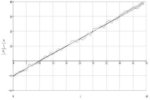
Fig. 1. Graphs of series: “clear”, with noise and restored

Noise clearing is W = 11.4% of the initial interferences.

• Example 2.    A series with periodicals, average interferences:

( i - 60)

• x, = —------- + 5sin ( i );

ⁱ 100

I = 0, 1, …, 59; N = 60; L = 30.

R i is a random value with uniform distribution from the interval [–3; 3].

Matrix S has dimensions of 30×30 and 30 eigenvalues λ _i (tab. 2).

Grouping of ones indexes from 27-th to 30-th is chosen, as corresponding to the most significant components. Elementary matrixes V 27 , V 28 , V 29 and V 30 correspond to them. Calculating the diagonal averaging for resultant matrix Y ^o = V 27 + V 28 + V 29 + V 30 , we get the restored series (fig. 2).

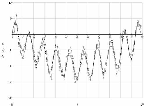
Fig. 2. Graphs of series: “clear”, with noise and restored

Noise clearing is W = 25.6 % of initial interferences.

Example 3. A series with several periodicals, high interferences:

x i = 0.03 i + 1.6sin (0.3 i + 0.17) + 1.3sin (2 i + 0.57);

I = 0, 1, …, 49; N = 50; L = 15.

R i is a random value with normal distribution, σ = 3 .

Matrix S has dimensions 15 × 15 and 15 eigenvalues λ i (tab. 3).

In this situation due to the high interferences the choice of components for the grouping is inconvenient, and to recognize a trend and periodicals is difficult. The analysis has shown that the increase in index quantity in a similar situation results in the restoring of not only an additive component, but also that of non-separated noise.

Table 1

The contribution of eigenvalues λ _i of matrix S , in percentage of their sum

i	1	2	3	4	5	6	7	8	9	10	11	12	13
λ i , %	0,00	0,00	0,00	0,00	0,00	0,00	0,01	0,01	0,01	0,00	0,01	0,01	0,01
i	14	15	16	17	18	19	20	21	22	23	24	25
λ i , %	0,02	0,02	0,02	0,02	0,03	0,03	0,03	0,04	0,08	0,08	2,76	96,8

Table 2

The contribution of eigenvalues λ i of matrix S , in percentage of their sum

i	1	2	3	4	5	6	7	8	9	10	11	12	13	14	15
λ i , %	0,03	0,03	0,03	0,03	0,04	0,05	0,02	0,07	0,07	0,07	0,08	0,01	0,00	0,00	0,12
i	16	17	18	19	20	21	22	23	24	25	26	27	28	29	30
λ i , %	0,11	0,12	0,12	0,17	0,20	0,21	0,21	0,22	0,26	0,29	0,33	4,14	5,97	7,58	79,44

Table 3

The contribution of eigenvalues λ i of matrix S , in percentage of their sum

i	1	2	3	4	5	6	7	8
λ i , %	2,50	2,49	2,85	2,14	1,94	3,29	4,00	4,73
i	9	10	11	12	13	14	15
λ i , %	5,26	6,83	7,78	9,99	11,31	13,83	21,07

Noise clearing with the 3 most significant components is W = 21.8 % , for 4 it’s W = 29.2 % and for 5 it’s W = 34.6%.

The results for 3 selected components are shown below as graphs (fig. 3).

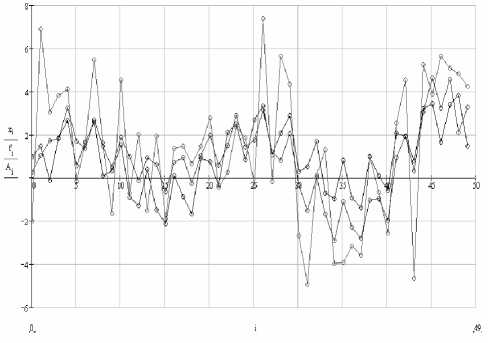
Fig. 3. Graphs of series: “clear”, with noise and restored

Concluding the given examples we can state that the basic algorithm of the “Caterpillar”-SSA method copes with the assigned task: for time series it separates trend and periodicals from interferences, reducing noise level down to 2–3 times; although the types of significant components aren’t defined, whether they are linear, periodic, logarithmic or other. This is an advantage of the method, which will make possible to create a powerful mechanism of non-parametric analysis of time series in the future, including computer programs.

The disadvantage of the basic algorithm is the necessity of manual intervention for the divided components analysis; also there is a problem in selecting the length of period and the quality of additive components division, depending on that. Further research will be dedicated to the automation of analyzing processes and other methods, improving the quality of the algorithm work results and reducing the manual aspect in this process.