Text classification using SVM enhanced by multithreading and CUDA

Published Online January 2019 in MECS DOI: 10.5815/ijmecs.2019.01.02

With the rapid growth and expansion of the internet, classifying digital text documents has been an area of constant research. Text classification can be used to categorize news articles, blog posts, open bulletin boards, online forums, etc. Text classification is essential as it helps find relevant information based on a user’s search string and helps associate one document with another. In recent times, Natural Language Processing (NLP), Machine learning and Data mining techniques work in tandem to automate text classification. Properly representing, annotating and summarizing presents various challenges – which need to be taken care of for an efficient and accurate classification.

Multithreading is a technique by which a piece of code or a set of instructions is used by multiple processors simultaneously, each at a different stage of execution, for achieving parallelism and thus reduce overall execution time of the program. Multithreading is very popular in the modern era with various CPUs of Intel and AMD providing this as a feature, with each consumer grade processor offering anywhere from 2 to 64 threads. This feature is specific for CPUs. Parallelism on Graphics Processing Units (GPUs) is gaining attention with each graphic processor die having thousands of cores. A core on a GPU is weaker than that on a CPU in the sense that they are not capable of executing complex instructions like stemming and lemmatization – but are highly optimized for crunching numbers – and when about three thousand cores work in tandem, numeric calculations become a breeze. The sheer number of cores on a GPU offers an amount of parallelism which is orders greater than what CPU cores can offer. nVidia – a manufacturer of GPUs, had created a platform called CUDA, which allows developers to harness the raw power of the cores on their devices. The authors have utilized both multithreading and the CUDA platform to massively decrease the overall execution time of their algorithm.

Classification of documents into a fixed number of predefined classes is the main objective of text categorization. A particular document may get classified into multiple categories, a single category or no category at all. This process of classification can be automated by using classifiers which need to be trained using labelled examples – this is called supervised learning [1].

Text classification has a wide scope of application, such as: relevance feedback, netnews filtering, reorganizing a document collection, spam filtering, language identification, readability assessment, sentiment analysis etc. Text classification can be used in the field of business decision making, medicine and so on.

• II.    Related Work

For the purpose of text classification [2], a lot of different methodologies are used as depicted in [3,4]. Naive Bayes classifier [5], k-nearest neighbor algorithms, Decision trees such as ID3 or C4.5, Artificial neural networks etc. being some of the approaches used. The authors have chosen Support Vector Machine (SVM) for this implementation. SVM by nature is binary classifier, and for classifying text into N-number of classes, special strategies needs to be used to make SVM work like an N-class classifier. SVMs are often referred to as universal classifiers in the literature. This is especially because, by the use of an appropriate kernel function, SVMs can be used to learn polynomial classifiers, radial basic function networks and many more. SVMs have a striking property that their ability to learn is unrelated to the dimensionality of the feature space. This allows generalizing data even in the presence of many features. Text documents have numerous features and since SVMs use overfitting protection, which does not particularly depend on the number of features, they have the potential to perform well in such situations. A document vector, representing a particular document would essentially be a sparse vector. Kivinen et. al. [6] have provided evidence that additive algorithms, which share a similar inductive bias like SVMs are suitable for solving problems related to sparse instances [1].

While some classification algorithms naturally permit the use of more than two classes, others are by nature binary algorithms (allows classifying into two classes); like SVM; these can, however, be turned into multinomial classifiers by a variety of strategies [15]. If there are N different classes, One-vs-Rest (OVR) type of classifier will train one classifier per class in total N different binary classifiers. For the i^th classifier, let the positive examples be all the points in class I (i.e. all the labels which has class i as its label), and let the negative examples be all the points not in class i. Let f i be the i^th classifier [15]. Making decisions means applying all classifiers to an unseen sample x and predicting the label i for which the corresponding classifier reports the highest confidence score:

f(x) = arg max f i (x), where ‘i’ varies from 0 to N

Although this strategy is popular, it is a heuristic that suffers from several problems. At first, the scale of the confidence values may differ between the binary classifiers. Moreover, even if the class distribution is balanced in the training set, the binary classification learners see unbalanced distributions because typically the set of negatives they see is much larger than the set of positives [16].

Another type of classification approach is One-vs-One (OVO) which is also known as all-pairs or All-vs-All classification. After building (N(N-1))/2 classifiers, one classifier to distinguish each pair of classes i and j. Each receives the samples of a pair of classes from the original training set, and must learn to distinguish these two classes [16]. Let fij be the classifier where class i were positive examples and class j were negative [15]. At prediction time, a voting scheme is applied: all (N(N-1))/2 classifiers are applied to an unseen sample and the class that got the highest number of "+1" predictions gets predicted by the combined classifier.

f(x) = arg max (∑ f ij (x)).

I          j

This is much less sensitive to the problems of imbalanced datasets but is much more computationally expensive and some regions of its input space may receive the same number of votes.

Viewed naively, OVO seems faster and more memory efficient. It requires O(N2) classifiers instead of O(N), but each classifier is, on average much smaller. If the time to build a classifier is super linear in the number of data points, OVO is a better choice.

• III.    Proposed Algorithm

The proposed algorithm, as discussed in this paper has two major segments, viz., training and classification.

A Algorithm: Training

• 1.    Collect labeled dataset

• 2.    Create the following empty arrays:

• a.  2D array, named data, to store the resultant

cleaned, tokenized documents

• b.  1D  array, named label, to  store labels

corresponding to each document.

• c.    1D array, named uniqueLabels, to store the unique labels present in the dataset

• 3.    For each document present in the dataset, do the following:

• a.    Convert the document to lower case

• b.    Tokenize the lower case document and generate the wordset

• c.    Remove the following from the wordset:

• i.    Punctuations

• ii.    Stopwords

• iii.    Custom stopwords based on training dataset (if required)

• iv.    Custom elements, such as numbers, roman numerals etc. as per requirement based on training dataset

• d.    For each word present in the wordset, do the following:

• i.    Tag the word with its corresponding parts of speech tag

• ii.    Perform stemming by finding out morphological root of the word using the parts of speech tag as one of the parameters

• iii.    Perform lemmatization on the stemmed word to generate clean word.

• iv.    Add the cleaned word to the cleaned wordset

• e.    Add the cleaned wordset to data array

• f.    If the label of the current document is not present in the uniqueLabels array, then add it.

• g.    Find out the index of the label of the current document in the uniqueLabels array and add that index to the label array. In this way, it is ensured that labels are represented in a numerical format.

• 4.    Save the uniqueLabels array to disk for the classification phase.

• 5.    Create a hashtable, named vocabulary, to store all the unique words present in all the documents.

• 6.    Create the following arrays, for CSR Matrix generation:

• a.    1D array, named indices, which stores the index of the current word in the vocabulary. This will store all the indices of the words present in all the documents one after the other.

• b.    1D array, named indPtr, to store the index pointers, which indicates the beginning and end of each document in the indices array. Initialize it by adding 0 to indicate the beginning of the first document.

• 7.    For each cleaned wordset in the data array:

• a.    For each word present in the current wordset:

• i.    Check whether the current word is absent in the vocabulary hashtable. If yes, then calculate the current length of the vocabulary hashtable, which will be used to represent this word numerically. Then, using this word as key and this numeric value as value, form the pair and add it to the vocabulary hashtable.

• ii.    Use the word as key to obtain the corresponding value from the vocabulary hastable and add it to the indices array.

• b.    Calculate the current length of the indices array and store it to the indPtr array to mark the ending of the current and beginning of the next document.

• 8.    Save the vocabulary hashtable to disk to use it during the classification phase.

• 9.    Generate the CSR Matrix using the indices, indPtr as parameters along with a special array which contains all ones and of the same length as the indices array, to denote that each of those words whose indices are stored have been encountered once in the document.

• 10.    Calculate the Term Frequency – Inverse Document Frequency using the CSR Matrix as parameter and generate TFIDF Transformed CSR Matrix.

• 11.    Train the SVM with Linear kernel using the Transformed CSR Matrix. As Linear SVM is a binary classifier, and here a multiclass classification is required, One-Vs-Rest (OVR or OVA) strategy is used for reducing the problem of multiclass classification to multiple binary classification problems.

• 12.    Save the trained classifier to disk for the classification phase.

• B.    Algorithm: Classification

• 1.    Collect test dataset. This dataset may or may not contain labels. If labels are present, it then can be used to test the accuracy of the classifier. In this implementation, labeled dataset is used for testing purposes.

• 2.    Create the following empty arrays:

• a.    2D array, named testData, to store the resultant cleaned, tokenized test documents

• b.    1D array, named testLabel, to store labels corresponding to each test document.

• 3.    Fetch the uniqueLabels array from disk, generated during the training process.

• 4.    For each document present in the test dataset, do the following:

• a.    Convert the document to lower case

• b.    Tokenize the lower case document and generate the wordset

• c.    Remove the following from the wordset:

• i.    Punctuations

• ii.    Stopwords

• iii.    Custom stopwords based on training dataset (if required)

• iv.    Custom elements, such as numbers, roman numerals etc. as per requirement based on training dataset

• d.    For each word present in the wordset, do the following:

• i.    Tag the word with its corresponding parts of speech tag

• ii.    Perform stemming by finding out morphological root of the word using the parts of speech tag as one of the parameters

• iii.    Perform lemmatization on the stemmed word to generate clean word.

• iv.    Add the cleaned word to the cleaned wordset

• e.    Add the cleaned wordset to testData array

• f.    Find out the index of the label of the current document in the uniqueLabels array and add that index to the testLabel array. In this way, accuracy of the classifier can be checked at the end of classification phase by comparing labels present in the testLabel array with the predicted labels.

• 5.    Fetch vocabulary hashtable from disk, generated during training phase.

• 6.    Create the following arrays, for CSR Matrix generation:

• a.    1D array, named indicesTest, which stores the index of the current word in the vocabulary. This will store all the indices of the words present in all the test documents one after the other.

• b.    1D array, named indptrTest, to store the index pointers, which indicates the beginning and end of each test document in the indicesTest array. Initialize it by adding 0 to indicate the beginning of the first test document.

• 7.    For each cleaned wordset in the testData array:

• a.    For each word present in the current wordset:

• i.    Check whether the current word is present in the vocabulary hashtable. If yes, use the word as key to obtain the corresponding value from the vocabulary hastable and add it to the indicesTest array.

• b.    Calculate the current length of the indicesTest array and store it to the indptrTest array to mark the ending of the current and beginning of the next test document.

• 8.    Generate the CSR Matrix using the indicesTest, indptrTest as parameters along with a special array which contains all ones and of the same length as the indicesTest array, to denote that each of those words whose indices are stored have been encountered once in the test document. During this, the dimensions of the matrix should be equal to [length of testData array, length of vocabulary hashtable], to make the number of features used during training and classification phases the same.

• 9.    Calculate the Term Frequency – Inverse Document Frequency using the CSR Matrix as parameter and generate TFIDF Transformed CSR Matrix.

• 10.    Fetch the classifier from disk, generated after the training phase.

• 11.    Use the classifier to predict labels for each test document, using the Transformed CSR Matrix as parameter.

• 12.    Compare the predicted labels with the labels present in the testLabels array to calculate the accuracy of the classifier.

The algorithm which is discussed before has various components as depicted below:

• 1)    Pre-processing

Before the documents can be used in the algorithm, some preprocessing is required. First, the documents need to be converted into lower case. This is done so that words like “Test” and “test” are treated as the same word. Next, the document is tokenized to generate the wordset, so that each word, punctuation, numbers can be identified separately. For this, word_tokenize() method of ntlk.tokenize module is used. As opposed to this, had string.split() method, based on spaces, been used, the string, “Welcome, Hello World!” would have resulted in 3 tokens, viz., “Welcome,” , “Hello” and “World!” which does not serve the purpose. word_tokenize() would result in 5 tokens, viz., “Welcome”, “,”, “Hello”, “World” and “!” from which each word, punctuation can be identified separately.

Now, punctuations need to be removed from the wordset as they are useless during classification. Next, stopwords need to be removed from the wordset. Some extremely common words which would appear to be of little value in helping select documents matching a user need are excluded from the vocabulary entirely. These words are called stop words [17]. Custom stopwords can also be removed if the dataset demands for it. For example, words like “volume”, “edition”, “part”, etc. can also be treated as stop words in the context of book name classification as they possess no actual benefit to the classification process.

• 2)    Stemming and Lemmatization

In linguistic morphology and information retrieval, stemming is the process of reducing inflected (or sometimes derived) words to their word stem, base or root form—generally a written word form. The stem need not be identical to the morphological root of the word; it is usually sufficient that related words map to the same stem, even if this stem is not in itself a valid root.

For grammatical reasons, documents are going to use different forms of a word, such as organize, organizes, and organizing. Additionally, there are families of derivationally related words with similar meanings, such as democracy, democratic, and democratization. In many situations, it seems as if it would be useful for a search for one of these words to return documents that contain another word in the set.

The goal of both stemming and lemmatization is to reduce inflectional forms and sometimes derivationally related forms of a word to a common base form.

• 3)    Bag-of-words Representation

The   bag-of-words   model is a simplifying representation used in natural language processing and information retrieval (IR). In this model, a text (such as a sentence or a document) is represented as the bag (multiset) of its words, disregarding grammar and even word order but keeping multiplicity [21]. The bag-of-words model is commonly used in methods of document classification where the (frequency of) occurrence of each word is used as a feature for training a classifier.

For example, two simple text documents are considered here:

• 1.    John likes to watch movies. Mary likes movies too.

• 2.    John also likes to watch football games.

Based on these documents, vocabulary (i.e. list of words) can be constructed as:

[

"John", "likes", "to", "watch", "movies", "also", "football", "games", "Mary", "too"

]

In practice, the Bag-of-words model is mainly used as a tool of feature generation. After transforming the text into a "bag of words", various measures to characterize the text can be calculated. The most common type of characteristics, or features calculated from the Bag-of-words model is term frequency, namely, the number of times a term appears in the text. For the example above, the following two lists can be constructed to record the term frequencies of all the distinct words:

• (1 ) [1, 2, 1, 1, 2, 0, 0, 0, 1, 1]

• (2 ) [1, 1, 1, 1, 0, 1, 1, 1, 0, 0]

Each entry of the lists refers to count of the corresponding entry in the list (this is also the histogram representation). For example, in the first list (which represents document 1), the first two entries are "1,2". The first entry corresponds to the word "John" which is the first word in the list, and its value is "1" because "John" appears in the first document 1 time. Similarly, the second entry corresponds to the word "likes" which is the second word in the list, and its value is "2" because "likes" appears in the first document 2 times. This list (or vector) representation does not preserve the order of the words in the original sentences, which is just the main feature of the Bag-of-words model. This kind of representation has several successful applications, for example email filtering [21].

This can be represented using a 2D array as:

1 21120001 1"

.11110 1110 0.

Where row index denotes the document number and column index denotes the word index in the vocabulary. Whenever a word is encountered in a document, element present in that particular index [row, column] is incremented. All non-zero values in that matrix denote the number of occurrences of the word in a document.

As most documents will typically use a very small subset of the words used in the total dataset, the resulting matrix will have many feature values that are zeros. For instance, a collection of 10,000 short text documents (such as emails) will use a vocabulary with a size in the order of 100,000 unique words in total while each document will use 100 to 1000 unique words individually. In order to be able to store such a matrix in memory but also to speed up algebraic operations a sparse matrix is used [22]. For the same, Compressed Sparse Row matrix or CSR Matrix is used in this implementation.

• 4)    Vocabulary generation using Hashtable

In this implementation, the vocabulary is constructed using a hashtable, where words are treated as keys and a numeric representation of that word as value to form every key-value pair. Unlike arrays, hashtables do not have any indices. So, the length of the hashtable before inserting the newly encountered word is treated as the numerical representation of that word.

As an example, the following two documents are considered:

• 1.    John likes to watch movies. Mary likes movies too.

• 2.    John also likes to watch football games.

This forms the vocabulary hashtable as : -

{

"John"                :“0”,

"likes"                  :“1” ,

"to"                     :“2”,

"watch"              :“3”,

"movies"            :“4”,

"also"                 :“5”,

"football"             :“6”,

"games"             :“7”,

"Mary"              :“8”,

"too"                 :“9”

}

Hashtable is used instead of an array is to improve the search-time complexity to O(1).

• 5)    CSR Matrix Generation

The compressed sparse row (CSR) or compressed row storage (CRS) format represents a matrix M by three (one-dimensional) arrays, that respectively contain nonzero values, the extents of rows, and column indices. It is similar to Coordinate list (COO) but compresses the row indices, hence the name. This format allows fast row access and matrix-vector multiplications (Mx). COO stores a list of (row, column, value) tuples. Ideally, the entries are sorted (by row index, then column index) to improve random access times. This is another format which is good for incremental matrix construction [23].

For example,

A matrix,

• "0   0   00"

0  2  04

• j0   О   01.

can be represented using CSR matrix as,

(1, 1)2

(1, 3)4

(2, 3)1

During the classification phase, while creating the CSR Matrix, the dimension should be set to [length of testData array, length of vocabulary hashtable], to make the number of features used during training and classification phases the same.

• 6)    Term Frequency – Inverse Document Frequency

Term frequency–inverse document frequency is a numerical statistic that is intended to reflect how important a word is to a document in a collection or corpus [18]. It is often used as a weighting factor in information retrieval, text mining, and user modeling. The TF-IDF value increases proportionally to the number of times a word appears in the document, but is often offset by the frequency of the word in the corpus, which helps to adjust for the fact that some words appear more frequently in general. Nowadays, TF-IDF is one of the most popular term-weighting schemes [24].

In this implementation, the normalized TF-IDF is stored as a CSR Matrix.

• 7)    Support Vector Machine

A support vector machine constructs a hyper-plane or set of hyper-planes in a high or infinite dimensional space, which can be used for classification, regression or other tasks. Intuitively, a good separation is achieved by the hyper-plane that has the largest distance to the nearest training data points of any class (so-called functional margin), since in general the larger the margin the lower the generalization error of the classifier [7,27].

• 8)    Multiclass Classification: One-Vs-Rest

This strategy consists in fitting one classifier per class. For each classifier, the class is fitted against all the other classes. In addition to its computational efficiency (only n_classes classifiers are needed), one advantage of this approach is its interpretability. Since each class is represented by one classifier only, it is possible to gain knowledge about the class by inspecting its corresponding classifier [28]. After an extensive trial and error testing, OVR Strategy was chosen for this algorithm. It was found that OVR strategy gives more accuracy for most of the datasets which were used for testing this algorithm. Working methodology of the OVR strategy is already explained earlier.

The algorithm which has been elaborated in the previous paragraphs has been enhanced with the uses of multi-threading and CUDA as described below:

• a)    Multi-threading

To implement multithreading, some changes need to be done in the previously proposed algorithms. In the step 3 of training and in the step 4 of classification algorithm, where each document is processed from the dataset, multithreading can be used, so that multiple documents can be processed simultaneously. Number of threads that can be created will depend upon the CPU capabilities. List of unique labels has to be a shared variable, because during training phase, whenever any of the threads finds a new unique label, it needs to add it to this list, and when one thread updates the unique labels list, all the other threads should get this updated list. So, updating unique labels list needs to be treated as a critical section, and lock needs to be acquired while entering this critical section and needs to be released while leaving. During testing phase, this critical section is not required as nothing will be added to the unique labels list. Each thread will be given a near equal subset of the dataset and will create their own data and labels array. At the end, individual arrays created by each thread needs to be merged to obtain the complete data and label array for the given dataset. To add this enhancement, the following changes needs to be done:

• 1.    Set number_of_threads according to the CPU Capibilites

• 2.    Set    data_per_thread    =    dataset_size    /

• 3.    Create dataQueue and labelQueue to store individual data and label arrays obtained by each thread

• 4.    Create a 1D array to store the list of threads

• 5.    Repeat for i varriying 0 to number_of_threads-1

number_of_threads

• a.    Calculate start_index = i * data_per_thread and end_index = ((i+1) * data_per_thread) -1. This start_index and end_index denote the start and end index of the dataset which the current thread (Thread ID i) will be working with.

• b.    Create a new thread and pass the folliwng: i as thread ID, dataset (including labels), start_index, end_index, dataQueue, labelQueue, type of thread - "Train" or "Test"

• c.    Add the newly created thread to the list of threads

• d.    Start the newly created thread.

• 6.    Increment i by 1

• 7.    Create a new thread and pass the folliwng: i as thread ID, dataset (including labels), start_index, end_index, dataQueue, labelQueue, type of thread - "Train" or "Test". start_index is calculated same as earlier, but end_index = dataset_size - 1. This thread is created outside of the loop, sperately, becasue, if dataset_size is not divisible by number_of_threads, then using the formula used above for end_index will miss out last few data.For this same reason, the above loop itirates one less time (0 to number_of_threads - 1 instead of 0 to number_of_threads).

• 8.    Add the newly created thread to the list of threads

• 9.    Start the newly created thread

• 10.    Do the following in the body of each thread, which all of the threads will execute:

• a.    For each document present in the provided subset of the dataset, given to the current thread, do the following:

• i.    Convert the document to lower case

• ii.    Tokenize the lower case document and generate the wordset

• iii.    Remove the following from the wordset:

• 1.    Punctuations

• 2.    Stopwords

• 3.    Custom stopwords based on training dataset (if required)

• 4.    Custom elements, such as numbers, roman numerals etc. as per requirement based on training dataset

• iv.    For each word present in the wordset, do the following:

• 1.    Tag the word with its corresponding parts of speech tag

• 2.    Perform stemming by finding out morphological root of the word using the parts of speech tag as one of the parameters

• 3.    Perform lemmatization on the stemmed word to generate clean word

• 4.    Add the cleaned word to the cleaned wordset

• v.    Add the cleaned wordset to data array of the current thread

• vi.    If type of thread is "Train":

• 1.    Check if the label of the current document is present in the uniqueLabels array or not. If yes, then aquire lock and then add it. After adding, release the lock.

• 2.    Find out the index of the label of the current document in the uniqueLabels array and add that index to the label array of the current thread.

• vii.    If type of thread is "Test":

• 1.    Check if the label of the current document is present in the uniqueLabels array or not.If yes, then add its index, if not, then add -1 to the label array of the current thread.

• b.    Aquire a lock, as another ciritical section is encountered. Put data and label array of the current thread to the dataQueue and labelQueue respectively. Release the lock.

• 11.    Wait for all threads to finish their work

• 12.    Fetch all individual data and label arrays created by al the threads from the dataQueue and labelQueue respectively and merge them together to obtain combined data array and label array

• 13.    Continue the original training and classification algorithm after this

• b)    GPU Parallelism using CUDA

CUDA or Compute Unified Device Architecture is a parallel computing platform and application programming interface (API) model created by nVidia. It enables programmers to use a CUDA-enabled GPU for general purpose processing – an approach termed GPGPU (General-Purpose computing on Graphics Processing Units). The CUDA platform is a software layer that gives direct access to the GPU's virtual instruction set and parallel computational elements, for the execution of compute kernels. CUDA supports programming frameworks such as OpenACC and OpenCL to simplify parallel programming of heterogeneous CPU/GPU systems.

GPU based parallel programming can increase the speed of some algorithms significantly. In this project, authors have tried to use GPU parallelism for the document processing phase, but that attempt was unsuccessful because CUDA only supports those data types which have fixed shapes of its own. Another place where GPU parallelism can be applied, is during creation of the CSR Matrix, which is the step 7 of both training and classification algorithm. Based on the GPU capabilities, number of threads and blocks has to be chosen. Each thread will be given a near equal subset of the data and label array and will create their own label, indPtr and indices array. At the end, individual arrays created by each thread needs to be merged one after another to obtain the complete label, indPtr and indices array for the whole dataset. During this process, the ordering of data is changed randomly based on thread execution. For this reason, label array is also sent to each thread and a new combined label array is created at the end. Vocabulary hashtable has to be created during this process. This has to be shared among all the threads. So, inserting any data into the hashtable has to be treated as a critical section. So, this operation has to be performed as an atomic operation. If CUDA is not available, OpenCL based GPU parallelism can also be used in this place a similar manner. If neither is available, a same kind of algorithm can be used using multithreading. To add this enhancement, the following changes needs to be done:

• 1.    Retrieve maximum capabilities of the GPU using cudaGetDeviceProperties function. This will provide maxThreadsPerBlock,      maxThreadsDimesnion,

• 2.    Set    data_per_thread    =    dataset_size    /

• 3.    Create indPtrQueue, indicesQueue and labelQueue to store individual indPtr, indices and label arrays obtained by each thread.

• 4.    Launch kernel where dimensions are set based on maximum GPU capibilites and send the data and labels array along with the value of data_per_thread and number_of_threads.

• 5.    Inside the kernel function, do the follwing:

maxGridSize and calculate the number_of_threads that will be created by multiplying values of maxTheadsDimension

number_of_threads

• a.    Calculate start_index = i * data_per_thread and end_index = ((i+1) * data_per_thread) -1. If

current_thread_id = number_of_threads - 1 (i.e. if the current thread is the last thread), then set end_index = dataset_size - 1. This is done, becasue, if dataset_size is not divisible by number_of_threads, then using the formula used before for end_index will miss out last few data.

• b.    Create a subset_data array from data array, from index number start_index to end_index.

• c.    Create two 1D arrays - indices and indPtr, which will be used to store relevant data for the current subset_data.

• d.    For each cleaned wordset in the subset_data array:

• i.    For each word present in the current wordset:

• 1.    Check whether the current word is absent in the vocabulary hashtable. If yes, then calculate the current length of the vocabulary hashtable, which will be used to represent this word numerically. Then, using this word as key and this numeric value as value, form the pair and add it to the vocabulary hashtable. Adding data to the hashtable has to be performed as an atomic operation.

• 2.    Use the word as key to obtain the corresponding value from the vocabulary hastable and add it to the indices array.

• ii.    Calculate the current length of the indices array and store it to the indPtr array to mark the ending of the current and beginning of the next document.

• e.    Put indPtr, indices & label array to the indPtrQueue,     indicesQueue     and

• 6.    Wait for all the threads to finish their operations.

• 7.    Add 0 to indPtr.

• 8.    Clear all the values of labels array.

• 9.    For each value in indPtrQueue, indicesQueue and labelQueue, do the following: Size of all the queues are same, so one element will be taken from each.

labelQueue array respectively. This operation needs to be performed as an atomic operation.

• a.    Append the current indices array fetched from indicesQueue to the existing indices array.

• b.    Append the current labels array fetched from labelsQueue to the existing labels array.

• c.    j = last_index_of (indPtr)

• d.    last_value = indPtr[j]

• e.    individual_indPtr = current indPtr array fetched from indPtrQueue

• f.    Repeat for k varying from 0 to size_of(individual_indPtr) – 1

• i.    indPtr[k+j] = individual_indPtr[k] + last_value

• 10.    Continue the original training and classification algorithm after this.

• IV. Test Cases

The testing phase makes use of four data sets out of which three are publicly available and the last dataset was collected from live twitter feeds.

The datasets are: -

• 1.    List of books from Library Genesis Project.

• 2.    20 news group dataset from scikit-learn.

• 3.    4 out of 20 categories in 20 news group.

• 4.    Twitter data set collected using Twitter Streaming API.

• A.    List of books from Library Genesis Project

Based in Russia, this is the largest and longest running currently openly available collection of ebooks. Headed by a team led by bookwarrior and Bill_G (of fiction torrent fame), they have several initiatives:

• i.    Over 1.5 million files of mainly non-fiction ebooks.

• ii.    An equivalent number of mainly fiction ebooks.

• iii.    20 million+ papers from journals of science, history, art etc.

• iv.    Comics, magazines and paintings; totally amounting to at least 100 TB. [29]

An SQL file is hosted by the Library Genesis Project which contains the list of books that they host. This file is open source and can be used by the community. It is licensed under Apache License version 2.0 [30]. This SQL file is used to fetch the names of the books which belong to certain subjects. The subjects which are taken into consideration are – Chemistry, Physics, Biology, Mathematics, Psychology and Computer Science. The training data set contains approximately 90,000 book names. Certain stop words, like “volume”, “part”, “edition”, etc. are stop words which specifically pertain to book names. Hence, such stop words have to be considered in the cleaning phase. Each label has to be denoted by a numeric value as SVMs can only work with numeric values. The names of subjects are converted into numeric values by the program reading it.

Another sheet containing hundred book names of each subject is created manually using publicly known books and saved as an Excel file. This data set is used to test the accuracy of the classifier. The book classifier correctly classified the books from the testing data set with an accuracy of nearly 76.77%.

• B.    20 News group dataset from scikit-learn

  The 20 newsgroups dataset comprises around 18000 newsgroups posts on 20 topics split in two subsets: one for training (or development) and the other one for testing (or for performance evaluation). The split between the train and test set is based upon messages posted before and after a specific date. [31] The training data set contains of 11,314 posts and the testing data set contains 7,532 posts. [32]. Against each post, there is an associated label which will be one of the 20 possible labels. Each of these twenty labels are internally represented as numbers, instead of strings as SVMs can only work with numeric data. There are unnecessary metadata like “summary”, “from”, “subject”, etc. which are not related to any topic whatsoever and only degrades the accuracy of the classifier. To improve the accuracy, these headers and footers are removed and then proceed as normal with creating the classifier. The accuracy of the classifier before removing the headers was 57.67% using an SVM with Linear kernel with One-Vs-Rest (OVR or OVA). The accuracy of the same dataset, using the same SVM and Linear kernel, but after removing the headers and footers, reached a significant 61.34%. To further improve the accuracy, standard stop words were removed. Since these are normal day to day posts, written by humans, there are no context specific stop words. To do this, the NLTK package contains a list of such standard stop words which occur very frequently in the English corpus. Each post is checked for words which are present in this list of stop words. After removing such stop words, an accuracy of 68.77% was achieved with the same SVM with Linear kernel with One-Vs-Rest (OVR or OVA).

• C.    4 out of 20 categories in 20 news group dataset from scikit-learn

Four of the 20 categories are considered for further testing. The four categories are – alt.atheism, soc.religion.christian, comp.graphics and sci.med. Here, two categories, viz., alt.atheism and soc.religion.christian are closely related to each other, which would help analyze how good the classifier is at correctly identifying posts from these two classes. This would help identify exceptionally well trained classifiers as only the best classifiers would be able to correctly classify posts from these groups – thus increasing the overall percentage which would be indicative of the fact that it is an efficient classifier. The other two classes, viz., comp.graphics and sci.med are totally unrelated and have been selected as a control setup for cases when the classifier might not have been properly trained. If a classifier routinely incorrectly identifies test data from these two categories then it can be safely concluded that the classifier has been trained improperly.

The training data set contains 2,257 posts and the test data set contains 1,502 posts when the afore mentioned 4 out of 20 categories are selected. The accuracy of an SVM with Linear kernel with One-Vs-Rest (OVR or OVA) using this training and test data set reached 82.16%.

• D.    Twitter data set collected using Twitter Streaming API

The Twitter Streaming APIs give developers low latency access to Twitter’s global stream of Tweet data. Public streams, which have been used in this implementation, are streams of the public data flowing through Twitter. These are suitable for following specific users or topics, and data mining. A streaming client will be pushed messages indicating Tweets and other events have occurred, without any of the overhead associated with polling a REST endpoint. The streaming process gets the input Tweets and performs any parsing, filtering, and/or aggregation needed before storing the result to a data store. The HTTP handling process queries the data store for results in response to user requests. The benefits from having a real-time stream of Tweet data make the integration worthwhile for many types of apps [33].

For the present research work, some popular categories were thought of, viz., Movie, Food, Politics and Sports. Then, probable related keywords were chosen for each category to make up a list of search strings for each category. These additional related terms or keywords help to find more sample tweets from the live feed. These four categories are clearly disjoint and will help increase the accuracy of the classifier. For example, Food and Politics are in no way related to each other, neither are Sports and Movie. Sure enough, there can be cases where a person has tweeted about a movie which is based on some sport; but those would be fairly rare. The list of keywords chosen for each category is as follows:-

• 1.    Movie- “hollywood”, “movie”, “actor”, “grammy”, “ironman”, “superman”, “spiderman”, “pokemon”, “captain america”, “tintin”, “the blacklist”

• 2.    Food- “food”, “cuisine”, “tasty”, “yummy”, “yum”

• 3.    Politics- “politics”, “political”, “vote”, “trump”, “obama”

• 4.    Sports- “sports”, “cricket”, “baseball”, “basketball”, “football”, “olympics”

This data collection process based on keywords was run on a Microsoft Azure Virtual Machine with a Python application running in four individual command prompts, one for each category. At the end of 48 hours, the data collected was assimilated and was put together and labelled as the training data set in a JSON file. This same process was run for another 24 hours, and at the end, the data was put together and labelled as test data also in JSON format. The total number of cleaned tweets in the training dataset resulted to 12 lakhs and the total number of cleaned tweet in the testing data set amounted to 8 lakhs. The data collection process lasted for 72 hours in total. This data set was biased more towards the “Politics” category. There were almost double or triple times the number of tweets of “movie” category in “politics” category. The other categories had more or less the same number of tweets.

The Twitter Streaming API returns a JSON object which contains a number of fields out of which there is a “text” field which contains the main tweet. The other fields are just meta-data like date of post, time, username, etc. The “text” field is in raw byte format, indicated by a “\b” right at the beginning of the text string. The string corresponding to the “text” field needs to be cleaned since it contains indicators like “RT” if it is a retweet, hashtags, links to external websites, special characters, emojis, etc.

The cleaning phase involves removing unnecessary links, special characters and other such substrings as mentioned afore. The following substrings are removed from the string corresponding to the “text” field:-

• 1.    New line characters are replaced with a single space.

• 2.    HTML sequences like & &alt; are removed using regular expressions.

• 3.    Twitter handles are removed using regular expressions. The string is searched for ‘@’. Anything following that is removed, unless a space is encountered, and the search process continues to the next substring.

• 4.    External links like http, https, www, ftp are also removed using regular expressions.

• 5.    Websites are removed by checking whether a dot (‘.’) exists in the third or the fourth position from the end of the string.

• 6.    The “\b” indicator at the beginning of the string is removed.

• 7.    The “RT” – retweet indicator is also removed.

• 8.    For hashtags, anything after the “#” symbol is considered as a word for further processing.

• 9.    Emojis are expressed in the string as hexadecimal characters which begin with “\x”. Such substrings are identified in the string and are removed. This also removes any unprintable characters that a Twitter user might have put in his tweet.

All these words are striped off of white spaces and are added to a list. This list now contains the cleaned words which are then added with a corresponding label. The label is the category currently under consideration. This results in a two-attribute format, where the first attribute denotes the list of cleaned words from the initial string and the second attribute denotes the category. A list of these tuples is created to get the final list for that category. This process is repeated for all the four categories. At the end of the cleaning process, four 2dimensional lists are created, each list for each category. All these lists are saved in a JSON file. This is what is fed into the rest of the program for the training as well as classification phases.

One key-value pair of this dataset is like:-

"President Trump and his majorities in the House and Senate regroup after failure to pass the health care bill": "Politics", where the tweet is the key and the category is the value.

• V.  Results and Discussion

• A. Accuracy Comparisons

For comparing accuracy, various classifiers are compared during testing. SVM with linear kernel with both OVO strategy and OVR strategy are compared in this manner. SVM with RBF and Polynomial kernel both were tested with OVR strategy, as OVO is not supported by API. Linear, RBF and Polynomial kernels are compared in this manner. SVM is also compared with many other classifiers which are inherently Multiclass classifiers, like K-Neighbors, Decision Tree, Random Forest, Ada Boost, Bernoulli Naive Bayes and Multinomial Naive Bayes Classifiers. From preprocessing to Transformed CSR Matrix generation using TF-IDF all the steps of this algorithm is followed for all the classifiers. Only the last step where the output of TF-

IDF is fed into the Linear SVM with OVR strategy is replaced with respective classifiers. Table 1 and table 2 demonstrate the corresponding outputs obtained. The results have been shown correct up to 6 decimal places.

Table 2. F1 Score and Accuracy in a scale of 0 to 1 for all the classifiers used for LibGen Books Dataset and Twitter Dataset

	LibGen Books Dataset		Twitter Dataset
	F1	Accuracy	F1	Accuracy
Linear SVM-OVO	0.488098	0.797979	0.936331	0.935820
Linear SVM-OVR	0.400390	0.767677	0.937314	0.936752
RBF SVM-OVR	0.392233	0.760943	-----	-----
K-Neighbors Classifier	0.348024	0.643098	-----	-----
Decision Tree	0.376014	0.690236	0.914752	0.913779
Ada Boost Classifier	0.427957	0.414141	0.887528	0.879945
Bernoulli NB	0.473471	0.741044	0.927057	0.926928
Multinomial NB	0.433427	0.686869	0.892711	0.893348

As seen from the previous tables, some of the classifiers failed for certain datasets, like polynomial SVM with OVR and random forest for both LibGen and Twitter dataset, RBF SVM with OVR and K-Neighbors for Twitter dataset. These classifiers failed after they consumed a lot of CPU and eventually ran out of memory in the testing environment used – AMD FX-6100 Hexacore processor with 10 GB RAM. They failed because of the size of the dataset could not be handled by the classifier in the given testing environment.

Figure 1 depicts a comparative study of the results as shown in table 1.

Table 1. F1 Score and Accuracy in a scale of 0 to 1 for all the classifiers used for 20 Newsgroup Corpus and 4 of 20 Newsgroup

	20 Newsgroup Corpus		4 of 20 Newsgroup
	F1	Accuracy	F1	Accuracy
Linear SVM-OVO	0.660234	0.671402	0.804991	0.813582
Linear SVM-OVR	0.675375	0.687732	0.812527	0.821571
RBF SVM-OVR	0.627826	0.658125	0.739714	0.766977
Polynomial SVM-OVR	0.184571	0.138078	0.731497	0.748336
K-Neighbors Classifier	0.054097	0.065454	0.658187	0.663782
Decision Tree	0.397888	0.406930	0.565576	0.579228
Random Forest Classifier	0.439937	0.452735	0.655613	0.667776
Ada Boost Classifier	0.403365	0.403365	0.664652	0.673103
Bernoulli NB	0.420290	0.448221	0.658187	0.663782
Multinomial NB	0.600471	0.634758	0.648719	0.708389

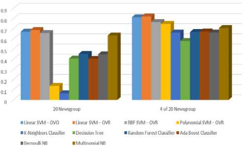
Fig.1. Accuracy comparison bar chart of various classifiers for 20 Newsgroup and 4 of 20 Newsgroup datasets.

20 Newsgroup consists of 20 different classes, so naturally the accuracy is less than 4 of 20 Newsgroup which contains 4 classes. Here, it is seen from figure 1 that for both the cases performance of Linear SVM with OVR is better than all the other classifiers.

LibGen books dataset was classified using various classifiers using same training and testing data given to all the classifiers. Only in this dataset, as depicted in figure 2, it can be noticed that the accuracy of Linear SVM with OVO is slightly better than OVR.

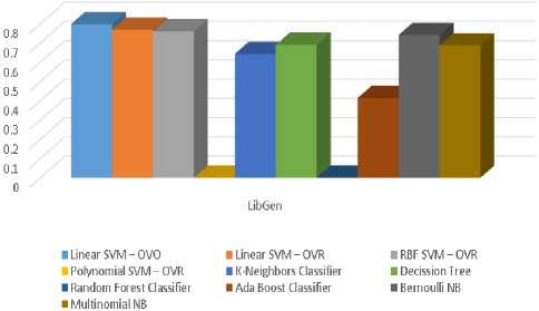
Fig.2 ． Accuracy comparison bar chart of various classifiers for LibGen dataset.

As seen from figure 3, Twitter streaming dataset gave very high accuracy in all the classifiers, because of the extensive cleaning processes the dataset has went through and also for the proposed algorithm.

Linear SVM with OVO and OVR gives almost the same accuracy as per the graph but the exact figures are OVO gives an accuracy of 0.935820206987 or about 93.4% where OVR gives 0.936752091088. So, it is noted that Linear SVM with OVR gives the most accurate result.

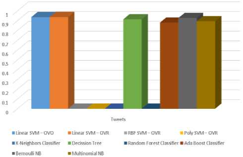
Fig.3. Accuracy comparison bar chart of various classifiers for Twitter streaming dataset.

B. Accuracy Comparisons

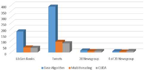
Fig.4. Execution speed comparison bar chart of base and enhanced algorithm for all the datasets

The originally proposed base algorithm was later enhanced using two enhancements - multithreading and GPU parallelism using CUDA.

For testing, at first, the base algorithm was executed. For the second test, the first enhancement, multithreading, was introduced. For the last test, both enhancements were used, i.e., multithreading and GPU parallelism. All the three tests were carried out on a Windows 10 Home Edition laptop with a dual-core Intel® Core ™ i3-2350M processor, clocked at 2.30 GHz with Hyper-Threading (enables it to have 4 threads), with 4 GB of RAM and nVidia® GeForce® 610M GPU with CUDA® compute capability of 2.1.

After all the three tests, it was observed that multithreading has increased the speed of execution at a significant level if the dataset is large (LibGen Books and Tweets). For smaller datasets (20 Newsgroup and 4 of 20 Newsgroup), the effect has not been that significant. After introducing GPU parallelism along with multi-threading, it was observed that for large datasets (LibGen Books and Tweets) execution speed has increased. But for small datasets like 20 Newsgroup, the execution speed decreases. For very small datasets like 4 of 20 Newsgroup, execution speed decreases significantly even worse than the base algorithm without any enhancements. For GPU parallelism using CUDA, data needed to be transferred from CPU to GPU and vice-versa. This extra overhead has caused the overall speed to decrease in case of small datasets. But for large datasets, the level of speed enhancement achieved has been more than the extra overhead, as there was a lot of data available to be worked on in parallel, so the overall execution speed has increased.

• VI.    Conclusion

While developing this system, a conscious effort has been made to create and develop a robust and efficient, making use of available tools, techniques and resources -that would generate an elegant system for automatic text classification.

• 10 GB of RAM, at an average of 8% CPU usage. All relevant statistics have been provided in the present paper.

Further improvements in execution time can be achieved by using GPU parallelism while creating the classifier object. As forethought, this approach can be used to classify YouTube videos, blogs, Facebook posts, or any other form of digital document. The classifier can be trained in a perpetual manner so that the classifier is aware of recent trending words. Similarly, data sets formed using previous decade's newspapers or blogs would provide an insight to archaic words to the classifier, like "bedlam", "demit", "dight" or "grimalkin" – which are no longer used frequently in the English corpus – and can therefore be used to classify old digital documents as well. Also, data sets provided by organizations like commoncrawl, which offer petabytes of data collected over more than 7 years of web crawling.

On a concluding note, the area of text classification is an ongoing research area and one could expect more efficient algorithms in the near future. With the size of the web ever increasing and the number of users skyrocketing, automatic text classification would be a pressing need felt by every single user.