Texture Analysis Based on Micro Primitive Descriptor (MPD)

Автор: Rasigiri Venkata lakshmi, E. Srinivasa Reddy, K. Chandra Sekharaiah

Журнал: International Journal of Modern Education and Computer Science (IJMECS) @ijmecs

Статья в выпуске: 2 vol.7, 2015 года.

Бесплатный доступ

Texture classification is an important application in all the fields of image processing and computer vision. This paper proposes a simple and powerful feature set for texture classification, namely micro primitive descriptor (MPD). The MPD is derived from the 2×2 grid of a motif transformed image. The original image is divided into 2×2 pixel grids. Each 2×2 grid is replaced by a motif shape that minimizes the local ascent while traversing the 2×2 grid forming a motif transformed image. The proposed feature set extracts textural information of an image with a more detailed respect of texture characteristics. The results demonstrate that it is much more efficient and effective than representative feature descriptors, such as Random Threshold Vector Technique (RTV) features and Wavelet Transforms Based on Gaussian Markov Random Field (WTBGMF) approach for texture classification.

Еще

Micro primitive descriptor, motif transformed image, texture classification

Короткий адрес: https://sciup.org/15014730

IDR: 15014730

Текст научной статьи Texture Analysis Based on Micro Primitive Descriptor (MPD)

Published Online February 2015 in MECS DOI: 10.5815/ijmecs.2015.02.05

The major role of Texture analysis and classification in many image areas, such as geo-sciences and remote sensing, medical imaging, stone texture classification, fault detection, image document processing and image retrieval. Texture is an exterior arrangement formed by uniform or non-uniform repeated patterns. It includes four fundamental problems: classifying images based on texture content; segmenting an image into regions of homogeneous texture; synthesizing textures for graphics applications; and establishing shape information from texture cue [1]. Texture discrimination or classification is the basis for many applications in computer vision. Texture classification has long been an important task in computer vision [ 2, 3, 4] by which different regions of an image are identified based on texture properties. It has been applied widely in different areas, such as medical image analysis [5], remote sensing [6], and biometrics [7]. Texture classification methods used can be categorized as statistical, geometrical, model based [2, 8, 9] and signal processing methods. Texture analysis aims at representing texture in a model that is invariant to changes in the visual appearance of the texture. The visual appearance of a single texture can change dramatically under the influence of, e.g., lighting changes and 3D rotations. Texture is characterized not only by the grey value at a given pixel, but also by the grey value pattern in an adjacent to the pixel.

At the beginning, extracting statistical feature to classify texture images, such as the co-occurrence matrix method [2] and the filtering based methods [10], is the main stream. Rotation invariance is a critical issue in many applications. In order to address it, many algorithms were proposed. Kashyap and Khotanzad [11] were among the first researchers to study rotationinvariant texture classification by using a circular autoregressive model. Later, many other models were explored, including the multiresolution autoregressive model [12], hidden Markov model [13], and Gaussian Markov random field [14].

The major step in description and classification of texture is study of patterns. For studying spatial structural and the textural characteristics of an image data various approaches are existed. [15], Fourier analysis for texture classification and noise removal [16, 17], fractal dimension for texture classification [18], variograms [19, 20, 21, 22] and calculating local variance for classification [23]. The most useful concept for dealing with regular patterns within image data is Fourier analysis. It has been used to clean out impair in radar data and to remove the special effects of regular undeveloped patterns in image data [24]. The basic fundamental tool for studying the regular patterns is local variance. It was carried out newly [25, 26]. Hence, the study of patterns still plays a significant area of research in classification, recognition and characterization of textures [27]. In [28], Ojala et al. proposed to use the local binary pattern (LBP) histogram for rotation invariant texture classification. LBP is a simple but efficient operator to describe local image patterns. Using a group of filter banks, Varma and Zisserman [29] proposed a statistical learning based algorithm, namely maximal response 8 (MR8), with which a rotation invariant texton library is first built from a training set and then an unknown texture image is classified according to its texton distribution. Zhenhua Guo et.al proposed a complex texton, complex response 8 (CR8)[30]. In this an 8-dimensional feature vector is extracted. After that, similar to MR8, a complex texton library is built from a training set by k-means clustering algorithm and then an texton distribution is computed for a given texture image[31]. In [31] proposed sparse representation (SR) method. In this A texton training dataset is first constructed by extracting patches in the training images, and then an over-complete dictionary of patch textons is learned from it under the SR framework By sparsely representing the texture image over the learned texton dictionary, a histogram of SR coefficients can be computed and used as features for texture classification. In [32] Laurens van proposed a 2D rotation method. In this method, image based textons are inclined to 2D rotations of the texture. It compares image-based textons with rotation-invariant textons based on spin images and polar Fourier features. The performance of this method is evaluated on the CUReT texture dataset for classification of Textures. Each of these methods depends upon how the texture features are selected for characterizes texture image. Whenever a new texture feature is derived it is evaluated whether it precisely classifies the textures or not. In the present paper, Textons are considered as micro primitive descriptor for texture classification. The different textons may form various image features. The present study attempted to classify various HSV-based color stone textures classification based on MPD histogram, which is different from the earlier studies. Based on the MPD the present paper evaluated a classification feature which is rotationally invariant.

The rest of the paper is organised as follows. Section 2 describes MPD detection method. The section 3 describes experimental results when the proposed method is applied. Comparison of the proposed method with other existing methods is discussed in section 5. The conclusions are given in section 5.

II. MPD Detection Method

Various algorithms are proposed by many researchers to extract color, texture and other features. Color is the most distinguishing important and dominant visual feature. That’s why color histogram techniques remain popular in the literature. The main drawback of this is, it lacks spatial information. Texture patterns can provide significant and abundance of texture and shape information. One of the features proposed by motifs patterns [33] called MPD, represents the various patterns of image which is useful in texture analysis. The proposed method consists of three steps which are listed below. In the first step of the proposed MPD evaluation, the color image is converted in to grey level image by using any HSV color model. The following section describes the RGB to HSV conversion procedure

Step1: RGB to HSV color model conversion In color image processing, there are various color models in use today. The RGB model is mostly used in hardware oriented application such as color monitor. In the RGB model, images are represented by three components, one for each primary color – red, green and blue. However, RGB color space is not sensitive to human visual perception or statistical analysis. Moreover, a color is not simply formed by these three primary colors. When viewing a color object, human visual system characterizes it by its brightness and chromaticity. The latter is defined by hue and saturation. Brightness is a subjective measure of luminous intensity. It embodies the achromatic notion of intensity. Hue is a color attribute and represents a dominant color. Saturation is an expression of the relative purity or the degree to which a pure color is diluted by white light. HSV color space is a non-linear transform from RGB color space that can describe perceptual color relationship more accurately than RGB color space. In this paper, HSV color space is adopted.

HSV color space is formed by hue (H), saturation (S) and value (V). Hue denotes the property of color such as blue, green, red, and so on. Saturation denotes the perceived intensity of a specific color. Value denotes brightness perception of a specific color. Thus it can be seen that HSV color space is different from RGB color space in color variations. When a color pixel-value in RGB color space is adjusted, intensities of red channel, green channel, and blue channel of this color pixel are modified. That means color, intensity, and saturation of a pixel is involved in color variations. It is difficult to observe the color variation in complex color environment or content. However, HSV color space separates the color into hue, saturation, and value which means observation of color variation can be individually discriminated. According to above descriptions about HSV color space, it can obviously observe that HSV color space can describe color detail than RGB color space in color, intensity and brightness. In order to transform RGB color space to HSV color space, the transformation is described as follows:

The transformation equations for RGB to HSV color model conversion is given below

V = max( R , G , В )	(1)
■ _ V—mm ( R , G , В ) V	(2)
H=— if V=R 6S ^J	(3)
H= +— if V=G 3 6S ^v	(4)
H= +R_G V=B 3 6S ^J	(5)

Where R, G, B are Red, Green, and Blue normalized in value [0, 1]. In order to quantize the range of the H plane is normalized with value [0, 255] for extracting features specifically

Step2: motifs texton pattern detection Texton-based texture classifiers classify textures based on their texton frequency histogram. The textons are defined as a set of blobs or emergent patterns sharing a common property all over the image [34, 35]. Based on the texton theory [34,

35], texture can be decomposed into elementary units, the texton classes of colors, elongated blobs of specific widths, orientation and aspect ratios, and the terminators of these elongated blobs.

The concept of ‘‘texton’’ was proposed in [34] more than 20 years ago, and it is a very useful tool in texture analysis. In general, textons are defined as a set of blobs or emergent patterns sharing a common property all over the image; however, defining textons remains a challenge. In [35], Julesz presented a more complete version of texton theory, with emphasis on critical distances (D) between texture elements on which the computation of texton gradients depends. Textures are formed only if the adjacent elements lie within the D-neighborhood. However, this D-neighborhood depends on element size. If the texture elements are greatly expanded in one orientation, pre-attentive discrimination is somewhat reduced. If the elongated elements are not jittered in orientation, this increases the texton-gradients at the texture boundaries. Thus, with a small element size, such as, 2×2 texture discrimination can be increased because the texton gradients exist only at texture boundaries [35]. In view of this and for the convenience of expression, the 2×2 block is used in this paper for textons detection.

There are many types of textons in images. In this paper, each texton is treated as a MPD. We only define six special types of motifs [33] textons for texture analysis. The six motifs are defined over a 2×2 grid, each depicting a distinct sequence of pixels starting from the top left corner as shown in Fig.1. In Fig.1 the six motifs are denoted as Z, N, U, C, Gamma and Alpha respectively. Each grid is scanned from top-left and those pixels formed a texton. Reverse direction of motifs are also considered. So, a total of 12 texton patterns are considered for texture classification. The first top-left six motifs of a 2×2 grid are shown in Fig. 1.

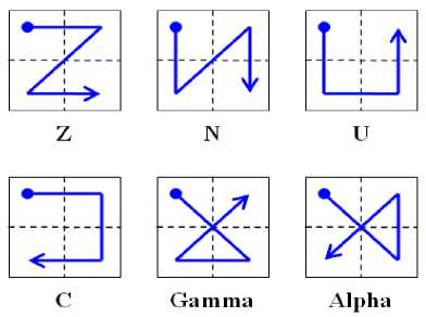
Fig 1. Six motifs texton of a 2×2 grid

Once the motifs are selected, the original image is divided into 2×2 grids. Each of the 2×2 grids contains four pixel values i.e., V 1 , V 2 , V 3 and V 4 . If the four pixel values of a 2×2 grid are distinct apply a suitable motif as in Fig.1 otherwise 2×2 grid will be zero. The working mechanism of MPD detection for the proposed method is illustrated in Fig.2.

202	53	149	54	255	254	253	124
78	55	84	52	57	190	186	250
129	68	35	128	160	38	36	255
183	29	140	68	54	31	144	182
176	52	47	43	47	53	145	156
145	38	61	45	47	62	140	176
150	186	188	188	220	211	87	167
99	196	189	174	155	159	151	106

(a)

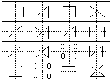
(b)

Fig 2. Example of motifs texton patterns a) 8×8 image b) motifs textons

Step 3: once the textons are identified The present paper evaluate the frequency occurrences of all six different textons (MPD) as shown in Fig.1 with different orientations. To have a precise and accurate stone texture classification, the present study considered sum of the frequencies of occurrences of all six different textons as shown in Fig.1 on a 2×2 block.

III. Results And Discussions

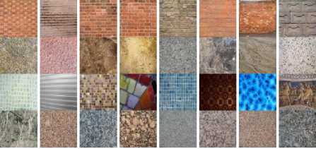
The present paper carried out the experiments on two data sets. The dataset 1 consists of various Brick, Granite, Marble and Mosaic textures with resolution of 256×256 collected from Brodatz textures, VisTex and also from natural resources from digital camera. Some of texture images in dataset1 are shown in the Fig. 3. The dataset 2 consists of various Brick, Granite, Marble and Mosaic textures with resolution of 200×150 collected from Outtex, CUReT database, and also from natural resources from digital camera. Some of texture images in dataset2 are shown in the Fig. 4.

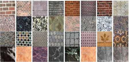
Fig 3. Input texture group of 8 samples of Brick, Granite, and Mosaic. Marble with size of 256×256

The frequency of occurrence of MPD of Brick, Granite, Marble and Mosaic texture images in dataset1 are listed out in Table 1, 2, 3, and 4 respectively. The sum of frequency of occurrence of MPD of each input texture images in dataset1 are listed out in Table 5. The Table 1, 2, 3, 4, 5 and the classification graph of Fig.5, indicates a precise and accurate classification of the considered stone textures.

Fig 4. Input texture group of 8 samples of Brick, Granite, Mosaic, Marble with size of 200×150

Tabble 1 Frequency occurrence of MPDs for brick textures in daraset1

SNO	Texture name	Z	N	U	C	Alpha	Gama
1	brick01	725	178	131	629	84	98
2	brick02	548	407	325	451	219	174
3	brick03	398	183	141	251	27	30
4	brick04	358	265	221	236	94	98
5	brick05	602	406	287	379	128	122
6	brick06	684	237	134	476	63	80
7	brick07	350	510	539	258	231	228
8	brick08	512	250	167	365	51	51
9	brick09	452	332	228	431	112	143
10	brick10	262	325	225	234	91	98
11	brick11	469	254	172	325	101	94
12	brick12	599	304	237	465	107	102
13	brick13	419	269	208	300	82	67
14	brick14	445	222	145	346	66	66
15	brick15	529	299	221	458	149	146
16	brick16	520	320	357	465	101	163
17	brick17	375	463	228	431	112	184
18	brick18	262	415	225	234	91	192
19	brick19	523	285	172	363	101	137
20	brick20	543	304	237	376	107	99

Tabble 2 Frequency occurrence of MPD for granite textures in daraset1

SNO	Texture name	Z	N	U	C	Alpha	Gama
1	granite01	2235	2803	564	442	49	44
2	granite02	2124	2433	704	566	78	89
3	granite03	2244	3056	609	409	43	50
4	granite04	2633	2668	698	708	89	92
5	granite05	1958	3298	944	630	129	113
6	granite06	2752	2541	739	762	99	99
7	granite07	2402	2686	790	717	108	116
8	granite08	2450	2532	739	732	108	98
9	granite09	2468	2252	599	597	78	78
10	granite10	2379	2925	768	706	104	126
11	granite11	2378	2290	602	585	83	88
12	granite12	2194	2526	957	863	195	178
13	granite13	1639	3264	650	316	41	37
14	granite14	2382	2323	724	755	89	82
15	granite15	2121	3121	885	664	108	114
16	granite16	2164	2903	1062	876	181	173
17	granite17	2431	2460	711	723	83	83
18	granite18	2523	2572	857	815	149	114
19	granite19	2270	2651	719	656	64	67
20	granite20	2165	2535	1168	1023	270	264

Tabble 3 Frequency occurrence of MPD for marble textures in daraset1

SNO	Texture name	Z	N	U	C	Alpha	Gama
1	marble01	1361	2173	273	200	14	18
2	marble02	2124	1672	417	520	55	44
3	marble03	2236	1339	210	300	12	17
4	marble04	2002	2108	598	535	66	70
5	marble05	2021	1986	475	505	65	56
6	marble06	2044	1924	448	474	57	49
7	marble07	1578	1351	221	252	22	18
8	marble08	1376	2376	460	231	17	28
9	marble09	2021	2383	347	344	19	24
10	marble10	1543	1772	277	276	26	21
11	marble11	1428	1717	376	328	37	27
12	marble12	2793	1559	435	772	80	90
13	marble13	1073	1859	490	235	44	59
14	marble14	457	3247	406	80	6	8
15	marble15	1654	2465	817	546	89	112
16	marble16	1984	2210	567	511	71	63
17	marble17	2211	2096	614	708	100	116
18	marble18	2124	1672	417	520	55	44
19	marble19	2044	1924	448	474	57	49
20	marble20	2021	2383	347	344	19	24

Tabble 4 Frequency occurrence of MPD for mosaic textures in daraset1

SNO	Texture name	Z	N	U	C	Alpha	Gama
1	mosiac01	774	790	370	376	131	139
2	mosiac02	799	817	348	343	104	106
3	mosiac03	891	688	318	378	109	119
4	mosiac04	664	577	350	326	129	137
5	mosiac05	860	857	535	493	237	218
6	mosiac06	953	891	385	414	252	252
7	mosiac07	1265	960	273	406	74	83
8	mosiac08	893	803	423	361	223	203
9	mosiac09	957	929	522	518	309	180
10	mosiac10	986	1005	533	487	206	186
11	mosiac11	905	897	537	554	257	290
12	mosiac12	1269	887	359	549	146	126
13	mosiac13	927	983	523	522	209	221
14	mosiac14	908	693	463	590	300	280
15	mosiac15	1078	910	435	549	148	161
16	mosiac16	940	911	403	392	120	107
17	mosiac17	793	729	378	374	154	150
18	mosiac18	911	752	431	561	217	218
19	mosiac19	1046	891	400	471	149	145
20	mosiac20	766	713	295	289	118	121

Tabble 5 Frequency occurrence of MPD for Brick textures in daraset2

SNO	Texture name	Z	N	U	C	Alpha	Gama
1	brick01	856	644	269	497	50	45
2	brick02	763	737	354	382	66	78
3	brick03	837	663	248	498	88	77
4	brick04	934	566	304	380	46	69
5	brick05	857	643	382	388	76	94
6	brick06	638	862	317	401	57	51
7	brick07	876	624	253	556	55	52
8	brick08	971	529	275	464	61	91
9	brick09	965	535	304	516	49	78
10	brick10	864	636	344	456	98	85
11	brick11	833	667	288	362	41	26
12	brick12	569	931	237	524	51	62
13	brick13	597	903	209	458	38	40
14	brick14	913	587	206	517	55	59
15	brick15	949	551	229	528	56	51
16	brick16	569	931	276	466	31	48
17	brick17	930	570	205	637	50	61
18	brick18	759	741	207	584	65	69
19	brick19	860	640	355	385	81	77
20	brick20	843	657	242	560	86	64
21	brick21	781	719	234	419	24	29
22	brick22	785	715	212	456	40	27

Tabble 6 Frequency occurrence of MPD for granite textures in daraset2

SNO	Texture name	Z	N	U	C	Alpha	Gama
1	granite01	598	902	458	571	173	181
2	granite02	530	970	465	450	158	191
3	granite03	687	813	455	425	141	123
4	granite04	692	808	441	458	137	123
5	granite05	751	749	517	432	136	145
6	granite06	988	512	391	601	117	122
7	granite07	909	591	523	458	149	158
8	granite08	805	695	508	483	167	180
9	granite09	802	698	425	578	123	146
10	granite10	569	931	414	492	149	143
11	granite11	731	769	220	590	96	102
12	granite12	845	655	412	496	133	144
13	granite13	972	528	488	533	177	147
14	granite14	864	636	397	464	112	104
15	granite15	762	738	503	483	152	165
16	granite16	876	624	454	428	174	170
17	granite17	850	650	408	367	178	92
18	granite18	694	806	270	549	96	90
19	granite19	846	654	433	438	107	96
20	granite20	921	579	481	327	123	80
21	granite21	945	555	418	456	116	96
22	granite22	936	564	529	469	151	164

Tabble 7 Frequency occurrence of MPD for Marble textures in daraset2

SNO	Texture name	Z	N	U	C	Alpha	Gama
1	marble01	753	747	582	556	256	256
2	marble02	680	820	539	563	230	241
3	marble03	693	807	624	509	226	218
4	marble04	756	744	585	547	216	203
5	marble05	876	624	527	545	178	162
6	marble06	963	537	589	479	182	194
7	marble07	534	966	523	537	204	203
8	marble08	576	924	550	506	204	192
9	marble09	667	833	556	509	214	208
10	marble10	765	735	611	529	231	226
11	marble11	772	728	584	583	266	270
12	marble12	861	639	616	570	269	273
13	marble13	963	537	605	588	285	291
14	marble14	861	639	570	578	278	268
15	marble15	888	612	517	565	205	191
16	marble16	723	777	574	547	248	234
17	marble17	693	807	626	401	209	191
18	marble18	794	706	665	503	248	250
19	marble19	815	685	638	512	245	263
20	marble20	914	586	713	481	237	214
21	marble21	813	687	577	472	178	216
22	marble22	971	529	665	522	265	268

Tabble 8 Frequency occurrence of MPD for Mosaic textures in daraset2

SNO	Texture name	Z	N	U	C	Alpha	Gama
1	mosiac01	896	604	239	290	56	58
2	mosiac02	675	825	257	255	23	33
3	mosiac03	824	676	213	218	8	22
4	mosiac04	867	633	82	72	3	1
5	mosiac05	610	890	276	199	12	15
6	mosiac06	725	775	135	169	16	19
7	mosiac07	795	705	226	282	49	62
8	mosiac08	595	905	135	202	6	9
9	mosiac09	535	965	92	91	6	6
10	mosiac10	634	866	236	238	37	37
11	mosiac11	916	584	318	288	46	24
12	mosiac12	827	673	119	140	8	6
13	mosiac13	809	691	188	223	43	42
14	mosiac14	907	593	260	305	27	33
15	mosiac15	506	994	155	157	6	7
16	mosiac16	632	868	2	392	5	3
17	mosiac17	681	819	331	175	77	72
18	mosiac18	781	719	41	38	5	5
19	mosiac19	786	714	178	125	9	8
20	mosiac20	985	515	188	251	94	70
21	mosiac21	927	573	165	203	10	14
22	mosiac22	765	735	80	90	1	2

1 2 3 4 5 6 7 8 9 10 11 12 13 14 15 16 17 18 19 20

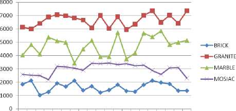
Fig 5. Classification graph of stone textures based on sum of the occurrences of texton

The Table 1, 2, 3, 4 and the classification graph of Fig.5, indicates that sum of frequency occurrences six texton features Z, N, U, C, Alpha and Gamma for Brick, Granite, Marble and mosaic in dataset1 textures are lying in-between 1030 to 2124, 5947 to 7367, 3442 to 5845, and 2183 to 3440 respectively.

The frequency of occurrence of MPD of Brick, Granite, Marble and Mosaic texture images in dataset2 are listed out in Table 5, 6, 7, and 8 respectively. The sum of frequency of occurrence of MPD of each input texture images in dataset1 are listed out in Table 10.

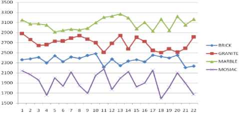
Fig.6: Classification graph of stone textures in dataset2 based on sum of the occurrences of texton

The Table 5, 6, 7, 8 and the classification graph of Fig.6, indicates that sum of frequency occurrences six texton features Z, N, U, C, Alpha and Gamma for Brick, Granite, Marble and mosaic in dataset 2 textures are laying in-between 2206 to 2484, 2505 to 2845, 2912 to 3269, and 1589 to 2176 respectively.

IV. Comparision With Other Existing Methods

The proposed motifs texton feature detection is compared with Random Threshold Vector (RTV) [36] and GMRF model on linear wavelets [37] methods. The above methods classified stone textures into three groups only. This indicates that the existing methods [36, 37] failed in classifying all stone textures. Further the present paper evaluated mean classification rate using k-nn classifier. The percentage of classification rates of the proposed method and crashes methods [36, 37] are listed in table 11. The table 11 clearly indicates that the proposed motifs texton feature detection outperforms the other existing methods and did not need any classification technique. Fig.7 shows the comparison chart of the proposed motifs texton feature detection with the other existing methods of Table 11.

Tabble 9 mean % classification rate of the proposed and existing methods

Image Dataset	Random Threshold Vector Technique	Wavelet Transforms Based on Gaussian Markov Random Field approach	Proposed Method (MPD)
Akar marble	93.29	92.19	94.56
VisTex	92.53	92.56	93.15
Outtex	93.30	93.29	96.57
Brodatz	93.59	92.86	95.06
CUReT	92.76	91.76	95.97

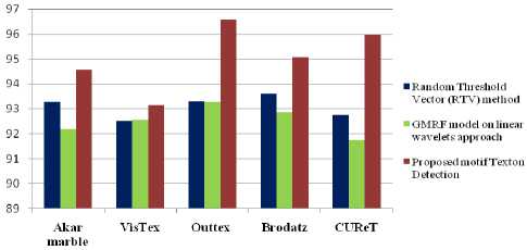
Fig 7. Comparison graph of proposed and existing systems

V. Conclusions

We proposed a new method, namely micro primitive descriptor (MPD), to describe image features for Texture classification which is rotationally invariant. The proposed MPD evaluates the relationship between the values of neighboring pixels. The proposed method has low time complexity and it is easy to implement. Textonbased texture classifiers form a new alternative to traditional texture classification approaches such as Markov Random Fields or filter bank models. The experiments were conducted on two datasets. The dataset consists of various Brick, Granite, Marble and Mosaic textures with resolution of 256×256 and 200×150 chosen from Brodatz, Vistex, Outtex, CUReT database, and also textured images from digital camera. From the graphs, it is shown that the frequency of MPD clearly classifies Brick, Marble, Granite and Mosaic textures. Recently Stone Texture Classification Based on Random Threshold Vector method classifies the Granite and Brick texture very clearly but this proposed method classifies 4 types of stone textures very clearly.

Acknowledgment

The authors wish to thank to all who are supported us while working in this research paper

Список литературы Texture Analysis Based on Micro Primitive Descriptor (MPD)

Bovik, A. C., Clark, M. and Geisler, W. S. "Multichannel texture analysis using localized spatial filters", IEEE Trans. Patt. Anal. Mach. Intell., 12, 1, pp. 55-73, 1990.
R.M. Haralick, K. Shanmugam, I. Dinstein, "Texture features for image classification", IEEE Transactions on System Man Cybernat, Vol. 8, No. 6, 1973, pp. 610-621.
Haralick, R. M. "Statistical and structural approaches to texture", Proc. of 4th Int. Joint Conf. Pattern Recognition, pp. 45-60, 1979.
Vijaya Kumar, V., Raju, U.S.N. , Chandra Sekaran , K. and Krishna, V. V. " A New Method of Texture Classification using various Wavelet Transforms based on Primitive Patterns", ICGST International Journal on Graphics, Vision and Image Processing, GVIP, Vol.8, Issue 2, pp. 21-27, 2008.
Jia, W., Huang, D.S., Zhang, D.: Palmprint Verification Based on Robust Line Orientation Code. Pattern Recognition 41(5), 1504–1513 (2008).
Anys, H., He, D.C.: Evaluation of Textural and Multi polarization Radar Features for Crop Classification. IEEE Transactions on Geoscience and Remote Sensing 33(5), 1170–1181 (1995).
Ji, Q., Engel, J., Craine, E.: Texture Analysis for Classification of Cervix Lesions. IEEE Transactions on Medical Imaging 19(11), 1144–1149 (2000).
M. Tuceyran and A.K. Jain, "Texture analysis, in Handbook of Pattern Recognition and Computer Vision", (2nd edition), World Scientific Publishing Co., Chapter 2.1, 1998, pp. 207-248.
F. Argenti, L. Alparone, and G. Benelli, "Fast algorithms for texture analysis using co-occurrence matrices", IEE Proceedings-F, Vol. 137, No. 6, December 1990, pp. 443-448.
Randen, T., Husy, J.H.: Filtering for Texture Classification: Pattern Analysis and Machine Intelligence 21(4), 291–310 (1999).
Kashyap, R.L., Khotanzed, A.: A Model-based Method for Rotation Invariant Texture Classification. IEEE Transactions on Pattern Analysis and Machine Intelligence 8(4), 472–481 (1986).
Mao, J., Jain, A.K.: Texture Classification and Segmentation Using Multiresolution Simultaneous Autoregressive Models. Pattern Recognition 25(2), 173–188 (1992).
Wu, W.R., Wei, S.C.: Rotation and Grey-scale Transform-invariant Texture Classification Using Spiral Resampling, Subband Decomposition, and Hidden Markov Model. IEEE Transactions on Image Processing 5(10), 1423–1434 (1996).
Deng, H., Clausi, D.A.: Gaussian MRF Rotation-invariant Features for Image Classification. IEEE Transactions on Pattern Analysis and Machine Intelligence 26(7), 951–955 (2004).
Richards, J. A. and Xiuping, J. (1999). Remote Sensing Digital Analysis: An Introduction. Germany: Springer- Verlag, vol.3, pp.363-363.
Moody, A. and Johnson, D. M. (2001). Land-surface phonologies from AVHRR using the discrete Fourier transform. Remote Sens. Environ., vol. 75, pp. 305-323.
Zhang, M., Carder, K. and Muller, karger. (1999). Noise reduction and atmospheric correction for coastal applications of landsat thematic-mapper imagery. Remote Sens. Environ., vol. 70, pp. 167-180.
Burrough, P. A "Multiscale sources of spatial variation in soil, the application of fractal concepts to nested levels of soil variation", Journal of Soil Sci., vol. 34, pp. 577-597. 1983.
Atkinson, P. M. and Lewis, P. (2000). Geostatistical classification for remote sensing: An introduction. Comput. Geo. sci., Vol. 26, pp. 361-371.
Curran, P. J. (1988). The Semivariogram in Remote Sensing: An Introduction. Remote Sens. Environ., vol. 24, pp. 493-507.
Treitz, P. (2001). Variogram analysis of high spatial resolution remote sensing data: An examination of boreal forest ecosystems. Int. J. Remote Sens., vol. 22, pp. 3895-3900.
Woodcock, C. E., Strahler, A. H. and Jupp, D. L. (1988). The use of variograms in remote sensing II: Real digital images. Remote Sens. Environ., vol. 25, pp. 349-379.
Moody, A. and Johnson, D. M. (2001). Land-surface phenologies from AVHRR using the discrete fourier transform. Remote Sens. Environ., vol. 75, pp. 305-323.
McCloy, K.R. (2002). Analysis and removal of the effects of crop management practices in remotely sensed images of agricultural fields. Int. J. Remote Sens., vol. 23, pp. 403-416.
Peder, Klith Bocher. and Keith, R. McCloy. (2006). The Fundamentals of Average Local Variance: Detecting Regular Patterns. IEEE Trans. on Image Processing, vol. 15, pp. 300-310.
Suresh A. and Vijaya Kumar V. et al. (2007). Texture Classification by Simple Patterns on Edge Direction Movements. International Journal of Computer Science and Network Security, vol. 7, no. 11, pp. 221-225.
Suresh A. and Vijaya Kumar V. et al. (2008). Classification of Textures by Avoiding Complex Patterns. Journal of Computer Science, Science Publications, USA, vol. 4(2), pp.133-138.
Varma, M., Zisserman, A.: A statistical Approach to Texture Classification from Single Images. International Journal of Computer Vision 62(1-2), 61–81 (2005).
Ojala, T., Pietik?inen, M., M?enp??, T.T.: Multiresolution Grey-scale and Rotation Invariant Texture Classification with Local Binary Pattern. IEEE Transactions on Pattern Analysis and Machine Intelligence 24(7), 971–987 (2002).
Zhenhua Guo, Qin Li, Lin Zhang, Jane You, Wenhuang Liu, and Jinghua Wang, "Texture Image Classification Using Complex Texton", ICIC 2011, LNAI 6839, pp. 98–104, 2012. Springer-Verlag Berlin Heidelberg 2012.
Jin Xie, Lei Zhang, Jane You and David Zhang , "TEXTURE CLASSIFICATION VIA PATCH-BASED SPARSE TEXTON LEARNING".
Laurens van der Maaten a Eric Postma a "Texton-based Texture Classification"
N. Jhanwar, S. Chaudhuri, G. Seetharaman, B. Zavidovique "Content based image retrieval using motif cooccurrence matrix", Image and Vision Computing 22 (2004) 1211–1220.
Julesz B., ―Textons, The Elements of Texture Perception, and their Interac-tions," Nature, vol.290 (5802): pp.91-97, 1981.
Julesz B., ―Texton gradients: the texton theory revisited," Biological Cybernet-ics, vol.54 pp.245–251, 1986.
B.V. Ramana Reddy, M.Radhika Mani, B.Sujatha, and Dr.V.Vijaya Kumar "Texture Classification Based on Random Threshold Vector Technique", International Journal of Multimedia and Ubiquitous Engineering Vol. 5, No. 1, January, 2010.
B.V. Ramana Reddy, M. Radhika Mani, and K.V. Subbaiah, "Texture Classification Method using Wavelet Transforms Based on Gaussian Markov Random Field" International Journal of Signal and Image Processing Vol.1-2010/Iss.1 pp. 35-39.

Еще

Статья научная

202	53	149	54	255	254	253	124
78	55	84	52	57	190	186	250
129	68	35	128	160	38	36	255
183	29	140	68	54	31	144	182
176	52	47	43	47	53	145	156
145	38	61	45	47	62	140	176
150	186	188	188	220	211	87	167
99	196	189	174	155	159	151	106

202	53	149	54	255	254	253	124
78	55	84	52	57	190	186	250
129	68	35	128	160	38	36	255
183	29	140	68	54	31	144	182
176	52	47	43	47	53	145	156
145	38	61	45	47	62	140	176
150	186	188	188	220	211	87	167
99	196	189	174	155	159	151	106

202	53	149	54	255	254	253	124
78	55	84	52	57	190	186	250
129	68	35	128	160	38	36	255
183	29	140	68	54	31	144	182
176	52	47	43	47	53	145	156
145	38	61	45	47	62	140	176
150	186	188	188	220	211	87	167
99	196	189	174	155	159	151	106