Texture Analysis of Remote Sensing Imagery with Clustering and Bayesian Inference

Published Online August 2015 in MECS DOI: 10.5815/ijigsp.2015.09.01

Texture is an important element for pattern recognition and interpretation in the human visual system. In a digital image, it represents the visual impression of smoothness or coarseness produced by the uniformity or variability of image color or tone [1]. Without universally accepted mathematical definition of texture, traditional approaches use symbolic descriptions, such as coarse and fine, rough and smooth, linear and nonlinear, low and high density, and orientation and directionality, etc., to represent texture in images [2]. However, descriptive terms for texture patterns presented in remote sensing imagery, usually generated by multispectral or hyperspectral sensors with various resolution, are yet to be established.

Texture analysis tools have been developed to extract features from remote sensing images with different criteria. The most frequently used pattern recognition techniques are built on statistical methods, such as spatial co-occurrence matrix and variogram. For instance, texture features are identified with a moving window to show the connection between a pixel and its neighbor according to a gray-level co-occurrence matrix (GLCM) [3]. Variogram analysis has been reported to be superior to GLCM for distinguishing very similar texture patches [4]. Algorithms based on the frequency transformation, such as discrete cosine transforms [5] and wavelet transforms [6] have achieved good performance in multiresolution texture analysis [7].

Texture features extracted from remote sensing images often offer complementary information for applications in which the spectral information of the images alone might not be sufficient for classifying spectrally heterogeneous ground cover and ground use classes [8]. Unsupervised classification techniques, such as morphology [9] and clustering [10], have been used to identify similar texture patterns in remote sensing images, with each pattern represented by a class that is labeled by domain experts in the post-clustering process. Another family of texture classification techniques have been developed from supervised classification methods, such as Bayesian classifier [11] and decision trees [12] when training data is available. Furthermore, Hybrid texture classification [13] involving multi-stage classification methods has demonstrated favorable results.

Extending this line of research, this study develops an application to extract texture features from remotely sensed images and classify the texture patterns with a new approach that integrates wavelet transformation, clustering, and probabilistic inference (See Fig. 1). To obtain the texture features, the Principal Component Analysis (PCA) [14] is performed on a multispectral Landsat TM image, with the first PCA component divided into regions of interest. The texture feature vector of each region is then represented by Gabor wavelets. The classification can be done in either online mode or batch mode. The online mode in which the feature vectors are directly fed into a binary Bayes Point Machine (BPM) [15] classifier allows the user to perform binary classification with dynamically created training data, while the batch mode supports multi-class classification, given the patterns of interest as well as training and testing data for the BPM classifier generated from an optimized k-means clustering method.

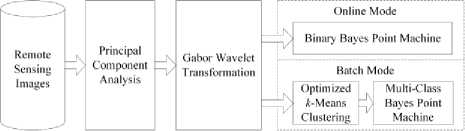
Fig.1. Remote sensing image texture extraction and classification.

The rest of the paper is organized as follows. Previous work related to this study is listed in Section II. Section III introduces the process of texture feature extraction by applying PCA to multi-spectral remotely sensed images and computing Gabor wavelets. The classification process that incorporates an optimized k -means clustering algorithm and a BPM classifier is presented in section IV. Section V deals with the implementation and the experiments, Section VI discusses the results in details, and section VII concludes with proposals for future work.

• II.    Related Work

Ref [16] compares the performance of various methods for multi-class texture image classification, such as Naïve Bayes classifier, k -nearest neighbor classifier and Neural Network classifier, given features represented by Haar wavelet. The results indicate the efficiency of using wavelet in multi-class texture image classification. In addition, a new texture classification method based on texton features, which evaluate the relationship between the values of neighboring pixels, has achieved better performance than existing methods on various stone textures [17].

Among unsupervised clustering algorithms, k -means clustering is popular due to its implementation simplicity and local-minimum convergence [18]. However, k -means clustering suffers some intrinsic deficiencies besides its expensive computation that requires multiple data scans to achieve convergence. For instance, it is very sensitive to initial starting conditions, i.e., k -means clustering is fully deterministic given the randomly or arbitrarily chosen initial centers. In addition, k -means clustering requires a parameter of the number of clusters, which is difficulty to obtain when no prior knowledge about the data is available. Although a general solution does not exist, various approaches have been proposed as partial remedies. For example, embedding the data set in a multiresolution kd -tree and storing sufficient statistics at its nodes may help to improve the speed of convergence [19]. A validity measure of clusters using intra-cluster and inter-cluster distance can be used to estimate the number of clusters [20]. Additionally, repeated sub-sampling and smoothing methods have been developed to refine the starting centers [21].

Recent advance in statistics learning with kernel methods has generated some powerful non-linear classification algorithms, such as Support Vector Machines (SVM) [22] and Bayes Point Machines [15]. SVM maximizes the margin between positive and negative training examples, the so-called support vectors, to find an optimal decision boundary, while BPM approximates the Bayes-optimal probabilities through the mass center of version space. These algorithms have performed well in the applications of content-based image retrieval [23], image classification [24, 25], and remote sensing image information mining [8].

• III.    Feature Extraction

• A. Principal Component Analysis for Satellite Imagery

Principal Component Analysis (PCA) is a coordinate transformation frequently used to reduce the correlation contained within a data set [14]. It has been applied to remote sensing image analysis to take out the correlation contained within the multispectral imagery by creating a new set of components, which are usually more interpretable than the original images. Ref. [26] provided a review of the applications of PCA in remote sensing, such as correlation analysis, change detection, and pattern recognition with multi-temporal Landsat TM images.

Assume N is the number of bands in a multispectral (multiband) remote sensing image, a pixel vector whose components are the individual spectral responses at a pixel location in each band can be characterized as x_k = [ X ], X ₂, — X_N У . PCA transformation computes the covariance matrix of the original data [26]

K

C x = -^fE ^{( x} k ^{- m}X^x k ^{- m ) T}         (1)

K ^{- 1} k = 1

where K is the total number of pixels and m = (1/ K ) ^ K x is the mean pixel vector. Given an identity matrix I , the eigenvalues X_k are computed via | C - ^ j| = 0 and the corresponding N -dimensional eigenvectors e that describe component axes are obtained from ( C - Л_к l ) e_A = 0 . As a result, the principal components are calculated by y_k = G ^T x_k where G ^T is the N x N orthonormal transformation matrix [26]

^G = ^[ e 1 , e 2 , —

6 11 e N ] T =    :

e N 1

. e 1 N ■" e NN

Each column in the transformation matrix represents the weights applied to the pixels in the corresponding band to create a principal component. The covariance matrix C of the transformed data becomes a diagonal matrix of which the elements are composed of the eigenvalues, while the transformed data points are linear combinations of their original data values weighted by the eigenvectors [26]. PCA component images built this way are uncorrelated and ordered by decreasing variance. The first component image, which has the largest percentage of the total variance and the highest signal-to-noise ratio, is used for texture feature representation.

B. Gabor Wavelet Transformation

Ref. [27] proposed a method for texture feature extraction based on Gabor wavelets, which may achieve the best overall performance compared with other multiresolution texture features using the Brodatz texture database. In addition, their experimental results on large aerial photographs indicate that Gabor wavelets give good accuracy of pattern retrieval [7].

A Gabor function and its Fourier transform are defined as [6]

For example, using three scales S = 3 and four orientations K = 4, a feature vector can be represented as f = [^00,^00, ^01,^01,™ ^23,^23 ]’         (9)

while the distance between images i and j in the feature space is [8]

d ( i , J ) = ZZ d mn ( г , J ) = 2Z mn      mn

¹ mn ^- ^ m п « ⁽ й _т„ )

( i ) mn

( j ) mn

« ⁽ ^ mn )

with the individual feature components normalized by a ( ^ _n) and a ( ^ „) , the standard deviations of the respective features over the entire set of images.

g ⁽ x , У ) =

1 I ----------I exp ^{2 п}^у J

- ^{1 f} — 7 + y " ^J + 2 n jWx

V —     У /

J ¹

G ( u , v ) = exp 4- —

( u - W )²

^ 2

v ²

+

Gabor wavelets, which form a self-similar filter dictionary, can be obtained by rotation and dilation of the Gabor function [27]

g mn ⁽ x , У ) = a - m g ⁽ x ', У ' ), a >  ¹ x ' = a ~^m ( x cos nn/ K , y sin nn/ K )

y ' = a~ ^m ( - x sin nn/ K , y cos nn/ K )         (5)

where m = 0,1,..., S - 1 and n = 0,1,..., K - 1 . S is the number of scales and K is the number of orientations in the multiresolution decomposition. The scale factor a ^{- m} normalizes the filter responses so that the energy is independent of m . Gabor filters are considered as orientation and scale tunable edge and line detectors, and the statistics of the filtered outputs can, therefore, be used to characterize the underlying texture information.

Gabor wavelet transform of an image I ( x , y ) is defined as [28]

• IV. Classification Methods

• A. Optimized k-means Clustering

An empirical comparison of initialization methods for k -means clustering was presented in Ref. [19]. This study adopts an optimized k -means clustering procedure [8] that combines the validity measure [20], which estimates the number of clusters, with initial centers refinement [21] based on repeated sub-sampling and smoothing.

Suppose N is the total number of pixels, K is the number of clusters, and x represents a texture feature vector, let m _; be the vector representing the center of cluster   C i ,  the validity of clusters is defined as

, where the intra-cluster distance        is intra      inter ,                                                        intra the average of the sum of distance between each vector and its cluster center, while the inter-cluster distance M is the minimum distance between any two cluster centers [20].

^Wmn ⁽ x , у ) = J ^{1 (} x 1 , У 1 ) g mn ⁽ x - x 1 , у - У 1 ) dx 1 dy 1     ⁽⁶⁾

where * indicates the complex conjugate. Suppose the local texture regions are spatially homogeneous, the mean and the standard deviation of the magnitude of the transform coefficients may represent the region for retrieval and classification [8, 28].

M mn ⁽ x , У ) = jj | ^Wmn ⁽ x , У ) |dxdy ⁽⁷⁾

^ mn ⁽ x , У ) = ^ jj ⁽ W mn ⁽ x , У )| ^- M mn ^ dxdy      ⁽⁸⁾

K

M inra =   ESI X - m i f         ⁽¹¹⁾

N i = 1 x e C i

M iner = m ⁿ| m i ^{- m} j| \\i = ^l - ² - ^ - ^{K -} 1, J = ^{г +} 1, - ^K

Assume K max is the upper limit of the number of clusters presented in a data set, for each integer k where 2 <  k <  K^ , the optimal number of clusters is found by clustering that yields clusters with the minimum validity.

The initial center refinement algorithm is briefly described as follows [8, 21]. Given randomly selected sub-samples Si■, i = 1, 2,^, J , k -means clustering may produce estimates of the true cluster centers CM i■ . A distortion value is computed as the sum of square distances of each data point to its nearest center. The centers with minimal distortion value over each subsample set are chosen as the refined initial centers. The algorithm also checks the solution at termination for empty clusters and sets the initial estimates of these

empty cluster centers to data points that are farthest from their assigned cluster center.

Algorithm 1 Optimized k -means clustering

Input: K , J , a dataset S = { x e X }

Output: K_opt , final hypothesis C

Begin for i = 1 … J do

Draw a random subset Si of S for k = 2 … K do

Mi

K ,= k with min —k-^nra-opt                              i k,Inter

Run k-means clustering on Si with K i to produce clusters Ci with centers CMi if Ci is empty else

^CM opt

= CM _i with min ^||x - CM, ||2 > _ ^{x e C} i

1 ^J

Run k -means clustering with K = — ^ Kⁱ and opt j^ opt

CM opt on S to output final hypothesis C

End

Bayes _z ( x ): = argmin E ,     ^[ l (H( x ), y ) ^{]          (15)}

yeY     HZ = z where the posterior probability is

Ph( h) PH|Zm = z (h) =| PH(V(z)) , 0, h e V (z) h g V (z)

given any prior belief P ( h ) . However, if the training data is limited, the optimal solution Bayes ( x ) may not be any single classifier h e H [29]. An approximation named Bayes point can be obtained through

[ e _h|_z m = z [ l ( h ( x ),H( x )) ] ]

h bp = Bayes bp ^{( z} ) ^: = arg min ^E X h e H

which implies the classifier h_bp e H is the best approximation of the optimal Bayes classifier on average over randomly sampled testing data [15]. For linear classifier, a hypothesis h ( _x ) _e H is defined by its weight vector w and therefore, h can be defined by w .

H :={x ^ sign ((x, w)), ||w|| = 1} (18)

The optimization procedure runs the cluster validation algorithm to find the optimal number of clusters K ⁱ for each sub-sample data set S i . The initial center refinement algorithm then uses K ⁱ to select optimized starting centers. The final clusters are generated by k -means clustering with K_opt which is the average of K ⁱ [8].

• B.    Bayes Point Machine Classification

A Bayes Point Machine (BPM) uses a hypothesis function h ( x ) to classify an input vector x by finding the inner product of x with a weight vector w , yielding the output y as true if the inner product w • x is positive and false otherwise [15]. Given training data z = ( x , y ) = ({ x , y }...{ x , y }) of size m , the hypothesis functions H form a version space V ( z ), with each point in V representing a possible classifier.

When the input distribution is spherically Gaussian,

f x ( x ) =

where d is the dimensionality of the feature vectors, the center-of-mass w in V can be a good approximation to the Bayes point [29]

w

cm

Ew_t m _{: i} [ ^{W ] E}»| z - = z [ W ]

Suppose y ' is the true output, a zero-one loss function may quantify the cost of predicting y

l o - i ⁽ У ^, У ' )

0,

1,

У = У' У * У'

The Bayes classification of test data h ( x. ) = y aims to minimize the loss [29]

Compared with other kernel based classifiers, such as SVM which aims to find the center of the largest sphere embedded in the version space V , with radius of the sphere being the maximal margin between positive and negative support vectors, the BPM looks for classification at the optimal center, i.e., the Bayes point, of the entire V . Therefore, SVM is an approximation to and theoretically less accurate than BPM [15].

• a. Binary BPM classification

integrated with other programming languages on Microsoft .NET, such as F#, for parallel computing.

Given the training data that consists of m feature vectors and        corresponding        observed        class labels D = {(x,, y.), i = 1,..., m} , the BPM classification aims to find the predictive distribution {p(y = c|x,D), c = 1,..., K} over K classes, conditional on x and D [30]. Assume a parametric density of the form p(y|x, w) = p(y|s = wT x) where 5 is the instance score, Fig. 2 illustrates that, the training of a binary BPM classifier learns a posterior distribution over the weight w, which is used in the predictions on testing data [30].

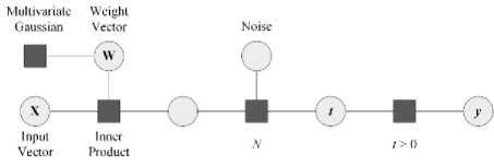
Fig.2. Factor graph of a binary Bayes Point Machine classifier (adapted from Ref [30] Minka, Winn, Guiver and Knowles).

Assume w is a vector with a multivariate Gaussian prior distribution, Gaussian noise is added to the score to allow for measurement and labelling error. Because if the training data is not linearly separable, which is common for kernel based classifiers, then no setting of w exists to classify the training data into two classes precisely. For each data sample during the training, variable t is computed by the inner product of w with the corresponding feature vector x in addition to the noise. The output variable y yields a value of true if t > 0 or false if t < 0.

• b. Multi-class BPM classification

The multi-class BPM classification is similar to the binary BPM classification. However, instead of using a single linear discriminant function, it has K functions with their respective weight vectors w c and scores s c , one for each class c in {1,..., K } [30]. The maximum score decides the class y to which a feature vector belongs.

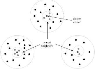
Fig.3. Training and testing data generated from nearest neighbors of the cluster centers.

The number of classes depends on the number of clusters generated from the optimized k-means clustering. Remote sensing domain experts may choose only the classes they are interested in. In addition, the training and testing texture feature vectors labeled by domain experts for multi-class BPM classification are built from the nearest neighbors of the cluster centers (See Fig. 3).

Assume M is the number of feature vectors in a cluster, the cluster center is computed as the average of all the feature vectors in that cluster.

MM

FC=Z fp =   Zlho °Po hPi <- hPop ]    (21)

p = 1               p = 1

The nearest neighbors of a cluster center are obtained by sorting the feature vectors according to their distance, e.g. the Euclidean distance, to the cluster center. The Euclidean distance between a feature vector and the q cluster center is defined as

d ( q , c ) =| F - f c |²= Z i, k a - a C ) ² + ^ - ^ ) ² ]   ⁽²²⁾

Algorithm 2 Multi-class BPM Classification

Training

Input: A set of clusters

Begin for i = 1 … K do for j = 1 … Mi do di ,j =||x-V" cm i| f

Train BPM with ( X , y ) to produce hypothesis

End

Testing

Input: A data set of

Output: Labeled data set

Begin

K

Run H on D to produce probabilities for t = 1 … N do

• ^x i , s = ^x t , У1 = ^l

Add ( x   , y ) to class D

End

• V.    Implementation and Experiments

• A.    Image Selection and Preprocessing

  The experiments were conducted on a geometric rectified Landsat TM image, which has a 30 meter by 30 meter spatial resolution for six of its seven bands. The PCA did not use the thermal-infrared band 6 because of its much worse spatial resolution of 120 meter by 120 meter. Fig. 4 shows the first PCA component image that consists of 4096 × 4096 pixels, covering the scene of middle Tennessee, USA. This image was then divided into 32 × 32 = 1024 regions of 128 × 128 pixels each.

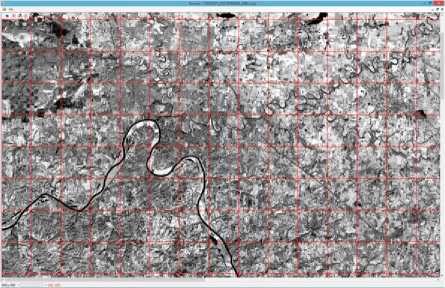
Fig.4. A Landsat TM image covering the scene of middle Tennessee (first PCA component).

For Landsat TM images, smaller region size may not cover sufficient spatial/texture information to characterize land use types, while a large region size may involve too much information from other types.

• B.    Feature Vector Construction and Clustering

  The Gabor wavelet feature vectors were computed using a C++ Dynamic Link Library (DLL) and imported to the optimized k -means clustering application developed with C# .NET. The filter parameters for Gabor wavelet were S = 3, and K = 4. The indices of the regions range from [0, 0] to [31, 31] for a total of 1024 regions.

The results of the optimized k -means clustering indicated the optimal number of clusters in the given image is 6. Fig. 5 shows the corresponding texture patterns identified by the clustering and labeled by a remote sensing domain expert.

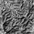
Deciduous/Evergreen Forest

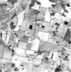
Raw Crops/Fallow

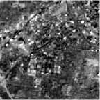
Residential/Industrial

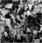
Grasslands/Herbaceous

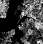
Water/Wetlands

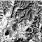
Pasture/Forest

Fig.5. Texture patterns identified by the optimized k -means clustering.

• C.    Binary Classification in the Online Mode

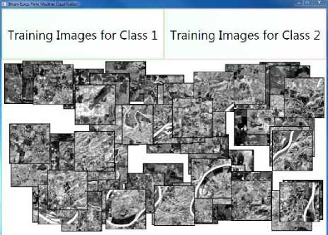
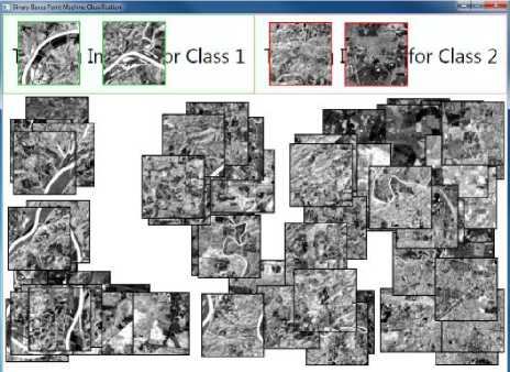
Based on the Image Classifier example of the Infer.NET [30], a binary BPM classifier running in the online mode was implemented to categorize only one of these texture patterns at a time. The experimental task for the binary classification was to find regions containing texture pattern of Water/Wetlands [31].

Fig. 6 demonstrates the classification process that involves user actions of dragging and dropping a region to the box for the corresponding class, which triggers an event handler to activate the training model of the binary BPM classifier. The rest of regions are categorized into two classes by the testing model of the BPM classifier. This classification process is animated by automatically moving a region to the side of the class it belongs to. How far to the left or right the region appears is a measure of the degree to which the binary BPM classifier believes it belongs to that class. It can be observed that more regions with Water/Wetlands are aligned to the left given more training images, and in the end, the majority of Water/Wetlands regions are correctly classified.

The binary BPM classification application has indicated the potential of the BPM classifier via an interactive visual presentation. However, quantitative measurements are desired according to the characteristics and size of the training and testing image set, as well as the classification accuracy [31], which is reported in the next section based on the experiments of the multi-class BPM classification.

• D.    Multi-class Classification in the Batch Mode

The multi-class classification was designed to run in the batch mode which takes a set of training images for the BPM classifier. Table 1 shows the total number of images labeled for each class based on the nearest neighbors of the cluster centers.

Table 1. Number of Images Labeled for Each Texture Class

Texture Class	Number of Images labeled
Deciduous/Evergreen Forest (D/EF)	150
Raw Crops/Fallow (RC/F)	110
Residential/Industrial (R/I)	130
Grasslands/Herbaceous (G/H)	110
Water/Wetlands (W/W)	80
Pasture/Forest (P/F)	120

Training image selection was done through an interactive user interface that allows the remote sensing domain experts to build a list of feature vectors with the associated regions (See Fig. 7). In addition, it offers a preview picture box to display the region when the user clicks on the file name in the list box. The testing results using 5-fold cross validation and 10-fold cross validation are presented in the following section.

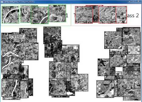
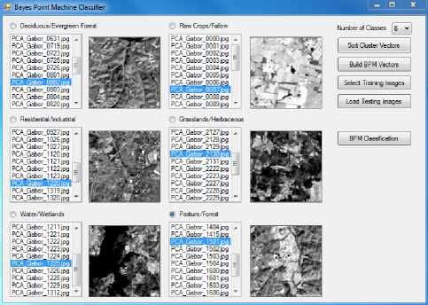
Fig.7. Training image selection for multi-class BPM classification.

• VI.    Results

  

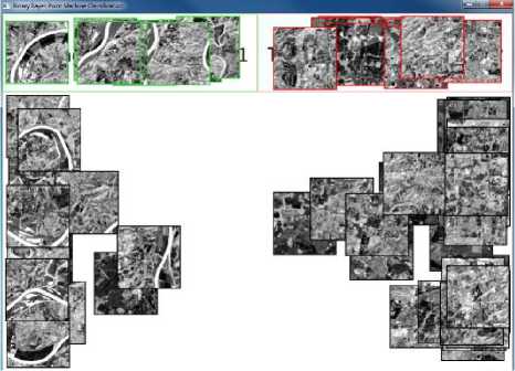
  Fig.6. An example of training and testing of the binary BPM classifier.

  
  

• A.    Classification Accuracy

Fig. 8 (a) demonstrates classification accuracy of each partition using 5-fold cross validation while Fig. 8 (b) shows classification accuracy of each partition using 10fold cross validation. It can be observed that the accuracy of Grasslands/Herbaceous (G/H) texture class is most consistent in each partition, while the accuracy of Water/Wetlands (W/W) texture class varies most significantly.

Meanwhile, the consistency of average classification accuracy of each texture class over all the partitions using 5-fold cross validation and 10-fold cross validation (see Fig. 9) indicates the effectiveness and robustness of the BPM classifier in multi-class classification.

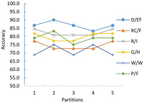
Fig.8. (a) Classification accuracy using 5-fold cross validation.

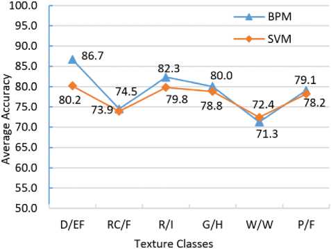
Fig.10. (a) BPM vs. SVM using 5-fold cross validation.

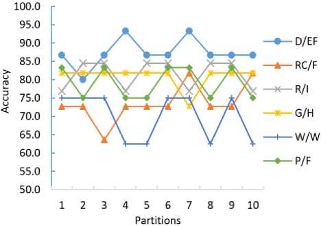
Fig.8. (b) Classification accuracy using 10-fold cross validation.

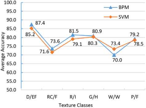
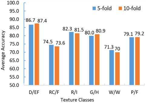
Fig.9. Average accuracy using 5-fold and 10-fold cross validation.

• B.    Comparing the BPM classifier with the SVM classifier

Additionally, using the same set of training and testing data, Fig. 10 (a) and (b) indicate the average accuracy of the BPM classifier compared with that of the SVM classifier implemented using LIBSVM [32] with 5-fold and 10-fold cross validation respectively. Overall, the BPM classifier achieved better results than the SVM classifier for all the classes except for Water/Wetlands, which is in line with the study that SVM is an approximation to and theoretically less accurate than BPM [15, 29].

Fig.10. (b) BPM vs. SVM using 10-fold cross validation.

The limited data size of the Water/Wetlands texture pattern may have caused the relatively low classification accuracy and led to this inconsistent performance. Meanwhile, the parameters of BPM and SVM classifiers were chosen based on the successful experience of previous studies [8, 31], which can be further adjusted and optimized.

• VII.    Conclusion

This study proposes a new approach for representing and extracting the texture features in remotely sensed images using PCA and Gabor Wavelets, and categorizing the texture patterns based on the BPM classifier and the adapted k-means clustering with estimated number of clusters and optimized initial starting centers. In particular, the training and testing data for the multi-class BPM classifier are obtained from the nearest neighbors of the cluster centers generated by the optimized k-means clustering, a unique process that may help the domain experts to select the texture patterns of interest and the corresponding training and testing regions in a large collection of images. The BPM classifier, when running in the online mode, provides the user an interactive visualization tool for binary classification. The experimental results of the multi-class BPM classifier running in the batch mode indicate overall good performance compared with the SVM classifier.

Our future work includes (1) create a database for better support of image selection and organization, (2) apply the proposed texture feature classification method to other types of satellite images, and (3) implement the algorithms in a parallel computing environment using F# programming language so that it scales well on larger set of images.

Acknowledgment

The authors thank Dr. B. S. Manjunath from University of California - Santa Barbara for sharing the C++ source code for the Gabor wavelet representation. This work is supported by the Scholarly and Creative Fellowship Program and the Presidential Research Scholars Program at Austin Peay State University.