The aircraft hydraulic system units and pipelines heat exchange parameters study

In the process of design and bench testing of an aircraft hydraulic system, a method of mathematical modeling of the thermal state of the hydraulic system is most applicable. The thermal state of the hydraulic system is determined by the temperature of the ambient air, the surfaces closely located to the hydraulic system components, by some other effects. The heat exchange parameters are determined by the thermophysical parameters of the units and pipelines of the hydraulic system, as well as by the topology of their location in the compartment. The mathematical model is developed according to the results of a flight experiment at the maximum ranges of flight parameters and outboard air conditions.

The mathematical model presents a system of partial differential equations for carbon-fiber composite thermal insulation together with ordinary differential equations for hydraulic system elements. A mathematical model identification requires effective methods for solving partial differential equations and ordinary differential equations, as well as methods of parametric identification. Besides, it is necessary to estimate the confidence intervals for each of the desired coefficients of the model.

Physical simulation of the thermal state of an aircraft hydrolic system units

The thermal state of the components of an aircraft hydraulic system is determined by the heat exchange between the outer surface of housings of the assemblies and pipelines and other close-located surfaces and ambient air. Besides, the thermal energy of the hydraulic system components is supplied and removed by the hydraulic fluid and the thermal control system.

The housings of the hydraulic system units and pipelines of the aircraft are coated with carbonfiber composite thermal insulation.

Mathematical simulation of the thermal state of an aircraft hydrolic system units

The mathematical model of the thermal state of the hydraulic system units is comprised of differential equations describing the heat exchange of carbon-fiber composite thermal insulation, and differential equations describing the thermal balance of the coating, of the air inside the compartment, of a pipeline or other component under review, of operational equipment [1–4]:

T_cov , t = 3 1 P v ( t ) V^ , _out ( t ) [T e ( t ) - T ( t )] -З 2 e ■ ( t ) [T_C o _V ( t ) - T_air ( t )] -

^-9 3 <

^Tcov ^{( t )}

T eq ( t ) 100

■^-& 4

^Tcov ^{( t )}

T eq , ef ( t )

+3 18 P ^{9 17} ( t )[T_e ( t ) - T cov ( t )] + 3 19

p _V ( t ) d p_V ( t )

T cv ( t )    d t

x [ T e ( t) - T co _V ( t )] + 9 21 Q cov , out

T ar , t = ^ 5 Г  ( t ) [T cov ( t ) - T ar ( t )] + $ 6 PC t ) [T cov ( t ) — T air ( t )] +

⁺$ 20 p^ dPT) [T cov ⁽ t ) — T ar ( t )] — $ 7 ^ ( t ) [T ar ( t ) — T eq ( t )] — T_cov ( t )    d t

—$ 8 P $ 17 ( t ) [T_a r ( t ) — T_eq , ef ( t )] + $ 22 .                                   (2)

T eq , t =$ 9 P $ ¹⁷ ( t )[ T r ( t ) — T eq ( t )] + $_W *

⁺ $ 11 *

T eq , ef ( t )

T eq ( t ) 100

T cov ( t ) 100

T eq ( t ) 100

H$ 12 ( T q - T eq )■

T eq , ef , t =$ 13 P $ 17 ( t ) [T ar ( t ) — T eq , ef ( t )] + $ 14 *

^Tcov ^{( t )}

—

T eq , ef ( t )

—

^—$ 15 *

T eq T eq , ef ( t )

T eq , ^{ef (} t )

^{> +} $ 16 •

where T –the temperature of hydrolic fluid circulating in a unit or a pipeline; T , T , T , T in expressions (1)–(4) with t index means time differentiation t of the temperature of the coating, the air inside the compartment, the thermal insulation surface of a unit or a pipeline, of operational equipment mounted close to the reviewed unit or pipeline respectively; p – outboard air density; 0 = [vj,u₂, .,u₁₇] ^T - vector of the model coefficients; T - superscript indicating the operation of transposition.

Instead of the calculated values a_eq of the heat transfer coefficient by convection of the unit or pipeline under review, the product of the measured air density overboard p V and the Mach number M of the aircraft in flight at M <  1 and the product p _V M² at M >  1is introduced.

In generalized form, the process of heat transfer in carbon-fiber insulation is described by the equations [5; 6]:

C cv ( x ) T_C v , t = ( X cv ( x ) T_C v , x ) x ,  0 <  x <  l , 0 <  t <  t k ;

^X cv ⁽ x ) F cv ^Tcv , x

= ^a cv , out ⁽ t ) F cv ^(Tcv ⁽ t , x ) ^— T air ⁽ t )) ⁺ Q cv , out ,      x = °i

^ cv ( x ) F  T

= a (t)F (T (t) — T (t,x)) + Q , х = Г, cv , n\ у cv \ cv , n\ у     cv\ , 77 cv-cv , in ,                ⁵

T cv (0, x ) = T o ( x ),  0 <  x <  l ,

where

C cv ( x ) =

'C compo ,   x ^{E co} mPo ,

C_air ,    x e air ,

X cv ( x ) =

^X compo ,   x ^{e cO} mPo ,

Xair,   x e air, where coefficients Ccv, X cv are determined by the examined layer of heat transfer.

In equations (5)–(8) the following notations are used:

Tcv(t, x) – thermal insulation temperature; Tcv,in (t) – temperature of the thermal insulation inner surface; T – first-order derivative T with respect to t ; T – first-order derivative T with re-cv,t                                            cv                                    cv,x                                            cv spect to x ; Tcv,x,x – second-order derivative Tcv with respect to x ; Ccv(x) – volumetric heat capacity or thermal insulation determined by the heat capacity of the composite Сcompo and heat capacity of the air Сair ; λcv(l) – thermal conductivity of the insulation determined by the composite thermal conductivity λ     and air heat conduction λ ; α     – heat transfer coefficient of the unit or pipeline out- compo                                     air     cv,out er surface; αcv,in – heat transfer coefficient of the unit or pipeline inner surface; Fcv – unit or piping surface area at external and internal heat exchange; Qcv,out – heat energy of external sources; Qcv,in – heat energy of internal sources; l – thickness of the thermal insulation layer.

Solution of the direct thermal state problem for hydraulic system elements

Ordinary differential equations (1)–(4) make up the following system:

Y t = F ( Y ( t , Θ )),   t ∈ (0, t t );   Y t = Y Θ ,   Y ∈ R^s ;   Θ∈ R^r ,                      (9)

where Y =[T  , T , T , T ]T – parameters vector of hydrolic system thermal state; Y – first-order derivative vector Y with respect to t .

The solution of the rigid system (9) of ordinary differential equations is proposed withing the following scheme applying Rosenbrock method [7]:

Yn+1=Yn+αK1+(1-α)K2;(10)

K1 =h(I-αhFY(Yn,tn,Θ))-1F(Yn,tn+αh,Θ);(11)

K2=h(I-αhFY(Yn,tn,Θ))-1F(Yn,tn+αK1,tn+2αh,Θ);  α =1-1/ л/2 ,(12)

where Y_n , Y_{n + 1} – solution of a system derived at n and ( n + 1) iterations, respectively; F – the right part of the system; F_Y – Jacobian matrix; I – identity matrix; h – integration step.

The solution of the system of differential equations with partial derivatives (5)–(8) is to be obtained in Monte Carlo method with smoothing coefficients in the form of mathematical expectation of the functional from the diffusion process [8–10].

Calculation of the diffusion process trajectories in the heat insulator cells is performed applying Euler method as random walk in moving spheres.

Parametric identification algorithm of mathematical simulation of an aircraft hydrolic system units’ thermal state

Coefficients vector Θ of the thermal state model of hydraulic system elements shall be determined by the minimum of function Φ ( Θ ) of weighted residual sum of squares [11] using iterative minimization algorithm:

N

Φ ( Θ ) = ∑ [ Y j - F ( Θ , U j )] ^TR ^- j ¹[ Y j - F ( Θ , U j )],                       (13)

j =1

где N – number of points over time; U – control vector; R_j – covariance matrix of uncertanties of heat exchange parameters.

Parametric identification of the thermal state mathematical model of hydraulic system units is to be performed by composition of the steepest descent method, Newton method, and quasi-Newton method of Broydon-Fletcher-Goldfarb-Shanno [12].

Estimation of mathematical model coefficients of hydrolic system units’ thermal state

The proposed theoretical method was applied to develop a mathematical model of the hydraulic system thermal state in an unpressurized aircraft compartment featuring a system of units and pipelines coated with carbon-fiber thermal insulation. The flight parameters and the overboard air conditions for the aircraft application model are shown in fig. 1.

The hydrolic fluid temperature up to 333 K serves as an optimization criterium of the modeled hy-drolic system coefficients. The air temperature in the compartment is up to 400 K.

T air,out ,

K

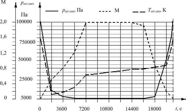
Рис. 1. Параметры режима полёта и воздушной среды за бортом модели применения летательного аппарата:

p air,out – давление воздуха за бортом за пределами теплового пограничного слоя;

M – число Маха н а внешней границе пограничного слоя; T air,out – температура воздуха за бортом за пределами теплового пограничного слоя

Fig. 1. Flight and outboard air parameters of the aircraft application model: p air,out – outboard air pressure beyond the thermal boundary layer; M – Mach number at the boundary layer outer threshhold; T air,out – outboard air temperature beyond the thermal boundary layer

Heat transfer coefficient of the carbon-fiber thermal insulation equals X cv =8-10 ² W/(m^K). Thickness of carbon-fiber thermal insulation l of the unit is taken as 2∙10^–2 m.

The obtained values of the model 0 coefficients of the unit are as follows: 0 =[1,258440^- 4   4,1542d0^-1    5,3417^10^-2    1,221540^-2    5,3456d0^-3

2,0357∙10–3         9,2045∙10–3    1,1904∙10–1    3,9123∙10–2    3,5162∙10–1

2,6877∙10–3         2,0979∙10–2    3,2077∙10–4    2,0343∙10–4    1,6850∙10–1

1,3344∙10^–4         5,1202∙10^–1] ^T .

Joint confidence intervals of the desired molel coefficients

At large dimension of the model 0 coefficients vector, the classical use of the joint confidence region [13] (Fig. 2) is associated with considerable problems.

For this reason, it was proposed to use joint confidence intervals Л0 * of coefficients in the form of joint confidence region projections onto coordinate axes of space 0 . This corresponds to replacing the hyperelliptic region with a hyperparallelepiped circumscribed around it. The following expression [14; 15] was derived for Л0 * :

Л& q =±,

X 2-a ⁽ r )

T ^, qq

q = 1,

] ;   ^Eq    ^Cq ^Dq ,

^Fq =[ e 1’ " e q -1 ¹ e q +1 • -- e r

D q   ^[ a 1 q-'-^a( q -1) q a ( q +1) q"' a rq ]   ^.

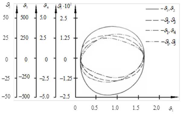
Рис. 2. Линии равного уровня функции невязки Ф (0) = 2734 вблизи действительных значений коэффициентов модели υ1,υ2,…,υ5

Fig. 2. Equal level lines of the residual function Ф (0) = 2734 close to the actual values of the model coefficients υ1,υ2 ,…,υ5

a 11--    1( q -1) a 1( q +1)   ”^1 r

^a(q -1)1 • " a ( q -1)( q -1) a ( q -1)( q +1) • a^a(q -1) r ^a ( q +1)1 • • - a ( q +1)( q -1) a ( q +1)( q +1) • " a ( q +1) r

ar 1 a.ar(q-1) ar(q+1)         a.drr where x2-a - distribution; Fq - (r x 1) - vector; Eq,  Dq - (r -1) x1 - vectors; Cq - (r -1) x (r -1) - matrix derived from matrix A by crossing-out q column of q line.

Here the estimates of confidence intervals A0 * of the coefficients obtained for the unit at confidence probability β = 0,95 are of the following values:

A0 * = [2,43394 0 6	4,5678∙10–3	2,7423∙10–5	6,5632∙10–3	3,2545∙10–5
4,5579∙10–5	2,2781∙10–6	1,9907∙10–3	8,5377∙10–4	3,4863∙10–3
6,3324∙10–6	4,6360∙10–4	4,6578∙10–7	3,2878∙10–6	5,5735∙10–4
3,7469∙10–6	7,4590∙10–5] T .

Conclusion

The paper presents a method of mathematical modeling of aircraft hydraulic system thermal state. The mathematical model is a system of partial differential equations for carbon-fiber composite thermal insulation together with ordinary differential equations for hydraulic system elements

The direct thermal state problem solution for hydrolic system elements elements, namely, the solution of a rigid system of ordinary differential equations, was performed with Rosenbrock method; the solution of a partial differential equations system was performed with Monte-Carlo method based on a probabilistic representation of the solution as a mathematical functional expectation of the diffusion process.

Parametric identification of the mathematical thermal state model of an aircraft’s hydraulic system components was performed with the composition of the steepest descent method, Newton method and quasi-Newton method of Broyden-Fletcher-Goldfarb-Shanno.

A mathematical model of the thermal state of a hydraulic system unit operating in an unpressurized aircraft compartment was developed, and the confidence intervals of each of the required model coefficients were estimated using χ ² distribution at confidence probability β = 0,95.