The Application of Bayesian Classification Theories in Distance Education System

Published Online July 2011 in MECS

In information systems, classification is one of the key parts for data mining. Such analysis can provide us with a better understanding of the important data classes and forecast future data trends. It is becoming important for individuation service to arrange associated training sessions and marketing strategy, according to individual demand and interest. Via the result of classifying, managers can arrange the associated training sessions and marketing strategy.

Self-Adaptive Learning System (SALS) can not only make the training projects based on the personalities and knowledge of learners, but also adjust the project according to the related facts automatically. The SALS is an integrated system including artificial intelligence, data mining, cognitive science, education, psychology, behavioral science and computer science. The purpose is to set up a dynamic adjustment model for individually education to meet the targets, behaviors, habits, preferences and situations of each student [1].

Distance Education System (DES) has two aspects of classifying target information – learning resources and learners. The learning resources are including the training courses, textbooks, coaching materials, and so on. By classifying the learning resources, the system can automatically provide some proposal of curriculum and evaluate the worth of courses.

In previous studies, Naïve Bayesian classification makes the assumption that the effect of an attribute value on a given class is independent of the values of the other attributes [2]. When the assumption holds true, then the naïve Bayesian classifier is the most accurate in comparison with all other classifiers. However, dependencies can exist between learning resources actually. Bayesian belief networks specify joint conditional probability distributions and allow class conditional independencies to be defined between subsets of variables. They provide a graphical model of causal relationships, on which learning can be performed [3].

In recent years, with the development of research, many researchers have made rich achievements in the application of Bayesian Networks. For example, Huang [4] introduced a construction method for university courses relationship Bayesian networks; Li [5] constructed a Bayesian network model for forecasting values of credit card customers; Leng [6] made a learning dynamic Bayesian network structure based on the basic dependency relationship between variables and dependency analysis method; Kelly [7] makes the prediction by the resource usage record;. In recent years, most of the distance education systems have become business system. During the fierce competition, it is absolutely vital to classify learners and to take pertinent marketing methods. This study presents a method based on the Bayesian networks for analyzing courses relationship and offering more support to make decision.

This article introduces a Bayesian networks classifier for classifying the learning resources and the relationship between courses. And a naïve Bayesian classifier is used in learner classification. Moreover, the managers can also use the result of classification to draw up the suitable curriculum for different learners. The rest of the paper is organized as follows. In Section 2 we will introduce the concepts of Bayes’ theorem, naïve Bayesian classification and Bayesian belief networks, while Section 3 presents a classifier model of learning resources and learners. Section 4 describes analytically the model simulation and system experiment. Finally, Section 5 concludes the paper.

• II.    Concepts of Bayes’ Theorem and Bayesian Belief Networks

• A.    Bayes’ Theorem

Bayes’ Theorem is named after Thomas Bayes, an 18th British mathematician and minister who did early work in probability and decision theory. Let X be a data tuple. It is usually described by measurements made on a set of n attributes. Let H be a hypothesis. P(H|X) is defined as a probability that the hypothesis H holds given the data tuple X . It is the posterior probability, or a posteriori probability, of H conditioned on X . In contrast, P(H) is the prior probability, or a priori probability, of H . Similarly, P(X|H) is the posterior probability of X conditioned on H and P(X) is the prior probability of X .

Bayes’ Theorem provides a way of calculating the posterior probability, P(H|X) , from P(H) , P(X|H) , and P(X) . Bayes’ Theorem is

_{P ( H | X ) =} P ( X | H ) P ( H )

P ( X )

.

For classification problems, let X be an observed data tuple, and suppose that H is the hypothesis that X belongs to a specified class C . We want to determine the probability P(H|X) that tuple X belongs to class C , based on the attribute description of X .

Bayesian classification is a statistical classified method. It can predict class membership probabilities, such as the probability that a given tuple belongs to a particular class. Both naïve Bayesian classifiers and Bayesian belief networks are based on Bayes’ theorem. They are useful in data mining and decision support.

• B.    Naïve Bayesian Classification

Naïve Bayesian classification, or simple Bayesian classification, assumes that the effect of an attribute value on a given class is independent of the values of the other attributes. It is made to simplify the computations involved and this assumption is called class conditional independence [2].

The naïve Bayesian classifier works as follows:

Let D be a training set of tuples and their associated class labels. Generally, each tuple is represented by an n -dimensional attribute vector, { x 1 , x 2 , … , x n }, depicting n measurements made on the tuple from n attributes, respectively, A 1 , A 2 , … , A n . Suppose that there are m classes, { C 1 , C 2 , … , C m }. Given a tuple, X , the naïve Bayes’ classifier will predict that X belongs to the class having the highest posterior probability, conditioned on X . That is the classifier predicts that tuple X belong to the class C_i if and only if

P ( C_i | X ) > P ( C_j | X ) for 1 ≤ j ≤ m , j ≠ i . (2)

Based on Bayes’ theorem,

P ( C i | X ) =

P ( X | C_i ) P ( C_i ) P ( X )

where P(X) is constant for all classes.

Thus only P(X|C_i)P(C_i) need be maximized. In other words, the predicted class label is the class C i for which

P(X|C i )P(C i ) is the maximum. That is

P ( X | C i ) P ( C i ) > P ( X | C j ) P ( C j ) for 1 ≤ j ≤ m , j ≠ i .

P(C_i) is the prior probability of C_i . It may be estimated by P(C i )=|C i,D |/|D| , where |C i,D | is the number of training tuples of class C i in D and |D| is the total number of training tuples of D .

It would be extremely computationally expensive to compute P(X|C i ) in given data sets with lots of attributes. In order to reduce computation, we make a naïve assumption that there are no dependence relationships among the attributes. Thus, n

P ( X | C i ) = ∏ P ( x k | C i )                           (5)

k = 1

= P ( x 1 | C i ) × P ( x 2 | C i ) × L × P ( x n | C i ).

The probability P(x_k|C_i) can be estimated easily from the training tuples. For each attribute, we should pay special attention to whether the attribute is categorical or continuous-valued.

If A k is categorical, then

P ( x k | C i ) = | A k , C_i |/| C i , D |,                        (6)

where | A_{k , C} |is the number of tuples of class C i in D having the value x k for A k , and |C i,D | is the total number of tuples of class C i in D .

If A k is continuous-valued, then the attribute is typically assumed to have a Gaussian distribution with a mean μ and standard deviation σ , defined by

1       _- ( x - µ ) ²

g ( x , µ , σ ) =         e ^{2 σ 2} ,               (7)

2πσ so that

P ( x_k | C_i ) = g ( x_k , µ _Ci , σ _Ci ).                (8)

• C.    Bayesian Belief Networks

Bayesian belief networks are also known as belief networks, Bayesian networks, and probabilistic networks. A Bayesian belief network is defined by two components: a directed acyclic graph and a set of conditional probability tables [2][8].

A Bayesian belief network is proposed with a triple, { N , E , P }. N is a set of nodes, N={x 1 , x 2 , … , x n } . In the directed acyclic graph, each node is representative a random variable and attribute. The variables and values may be discrete or continuous-valued. E is a set of directed edges, E={i, xj>|xi≠xj and xi, xj ∈N}. Each edge, i, xj>, represents a direct probabilistic dependence, that the reason (xi) points the result (xj). P is a set of conditional probability, P={P(xi | parents(xi))}. Each variable has one conditional probability table (CPT) in a belief network

Let X=(x 1 , x 2 , … , x n ) be a data tuple described by the variables or attributes Y 1 , Y 2 , … , Y n respectively. A Bayesian belief network provides a complete representation of the existing joint probability distribution with the following equation:

n

P ( x ₁, x ₂, L , x_n ) = ∏ P ( x_i | parents ( Y_i )) ^, i = 1

where P(x₁, x₂, … , x_n) is the probability of a particular combination of values of X , and the values for P(x i | parents(Y i )) correspond to the entries in the CPT for Y i .

Several algorithms exist for learning the network topology from the training data given observable variables. In this study, the construction algorithm of undirected graph based on information theory is used at first. Then, from the time order of courses, we can determine the direction of edge in the undirected graph. At last, the method of mathematical statistics is used to create the CPT.

A graph in which the nodes are connected by undirected arcs is called undirected graph. An undirected graph is an ordered pair, G= . N is a finite, nonempty set. The elements of N are called the notes of G . E , is a finite set of sets. Each element of E is a set that is comprised of exactly two notes. And the element of E is called edge of G .

• III.    A Bayesian Belief Networks Classifier Model of Learning Resources

• A.    The structure of Bayesian classifier model

In the DES, reforming the curriculum and learning materials is a very important task. At the beginning, the system manager may be use the previous experience in teaching. When the learning records in database accumulate enough to support the decision analysis, the Bayesian networks classifier can be used. The basic data resource for classification comes from two parts: firstly, the feedback of learning resources from the learners; secondly, the examination results of training courses.

To construct the Bayesian network of learning resources is a three-step process, as shown in Fig. 1. The first step constructs the undirected graph. The second step determines the direction of edge. The third step creates the CPT.

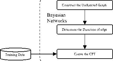
Fig.1 The graph of Bayesian networks construction

The learner classification is a two-step process, as shown in Fig. 2. The first step is the learning step, or training phase.

In the first step, the classification algorithm builds the classification rules by analyzing a training data set made up of training data tuples and their associated class labels.

The directed acyclic graph of the learning resources and the conditional probability tables, are computed based on the training data set.

The second step is the classification step. Given a target tuple, X , the classifier will predict the class label of X , by using the classification rules. The classifications have three aspects: firstly, according to the examination results determine the order of training courses; secondly, under the feedback of learning resources classification the learning resources grade; thirdly, the naïve Bayesian classifier is used to compute the customer value.

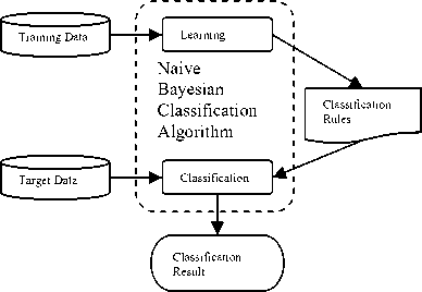
Fig.2 The structure graph of Nive Bayesian classifier model

• B.    The Undirected Graph Construction model

In the training of a Bayesian network, there are a number of scenarios. The majority of training methods are based on an advanced math background and a very complex computation. Here, information theory is used to construct a undirected graph.

In probability theory, two events X and Y are conditionally independent given a third event Z precisely, if the occurrence or non-occurrence of X and the occurrence or non-occurrence of Y are independent events in their conditional probability distribution given Z . In other words, X and Y are conditionally independent if and only if, given knowledge of whether Z occurs, knowledge of whether X occurs provides no information on the likelihood of Y occurring, and knowledge of whether X occurs provides no information on the like hood of Y occurring.

Symbolic probabilistic relational is given by

P ( X I Y | Z ) = P ( X | Z ) P ( Y | Z ) ,               (10)

or equivalently,

P ( X | Y I Z ) = P ( X | Z ) ,

In information theory, let U is the finite set. X , Y and Z are three subset of U and not intersect with each other. I(X, Y, Z) , named as mutual information, is used to express X and Y are conditionally independent with Z . When the event Z is given, the conditional mutual information of X and Y value as follows:

I ( X , Y | Z )

P ( x_i , y_j | z_k ) P ( x_i | z_k ) P ( y_j | z_k )^,

IJK

∑∑∑ P ( x_i , y_j , z_k )log i = 1 j = 1 k = 1

Let ε (a small positive real) is a threshold value. If I ( X , Y | Z ) ≤ ε , it means that X , Y and Z are conditionally independent, otherwise they are not conditionally independent.

The probabilities, P(x i , y j , z k ) , P(x i , y j | z k ) , P(x i | z k ) and P(y j |z k ) , may be computing by the data sample.

The algorithm proceeds as follows[4]:

• 1)    Input the data sample contained with n attributes and the threshold value, ε .

• 2)    Sequential search the attributes and test I(X, Y | Z) between the each two attributes of X and Y, where Z=U-X-Y .

• 3)    If I ( X , Y | Z ) > ε , there is an edge between X and Y, otherwise there is no edge between them.

• 4)    Output the undirected graph with all edges.

• C.    RFM customer relationship management model

Customer Relationship Management (CRM) is a philosophy of business operation for acquiring and retaining customers, increasing customer value, loyalty and retention, and implementing customer-centric strategies; enterprises can shorten sales cycle and increase customer loyalty to build better close relationships with customers and further add revenues by good CRM [9]. According to the research of Arthur Hughes [10], Recency, Frequency and Monetary model (RFM) is a simple and effective CRM method that differentiates important customers from large data by three attributes:

• 1.    Recency. How recently the customer has purchase.

• 2.    Frequency. How often the customer purchases during a particular period.

• 3.    Monetary. How much the customer spends during a particular period.

The RFM model can be used for predicting the customer value in most sales and business fields. With the progress of database technology and business intelligence, various kinds of RFM systems have emerged and are undergoing development to address the requirements of new applications. The value of customer, CV , can be computed as

CV = λ _rR + λ _fF + λ _mM            (13)

where the variables R , F and M is the value of the attributes recency, frequency and monetary, and the parameter λ r , λ f and λ m is the weights of the variables R , F and M . As usual, the weights are set by personal experience. Although it makes the calculation simple and fast, the result is not good enough to justify objectivity and impartiality.

In this paper, customers (or learners) are assigned a ranking number of 1, 2, 3, 4 or 5 (with 5 being the highest) for each RFM attribute. The naïve Bayesian classifier is used to compute the customer value.

• IV.    Model Simulation and System Experiment

• A.    Model Simulation

The classification of learning resources and training courses is a complex computation. In this paper, the test scores of learners are used as the sample set. Fig. 3 shows the undirected graph of training courses based on the information theory.

The courses type, course_type , has five distinct values (namely, { vocabulary , reading , listening , writing , speaking }). Therefore, based on three different level of courses (namely, { primary , intermediate , advanced }), there are fifty distinct courses type. Let course Cvp correspond to the primary vocabulary course, course Cvi correspond to the intermediate vocabulary course, course Cva correspond to the advanced vocabulary course, and so on.

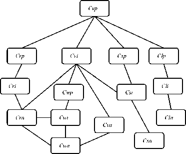
Fig.3 The Undirected Graph of Training Courses

In accordance with the time order of courses, the direction of edge in the undirected graph can be determined. Fig. 4 shows the Directed Acyclic Graph of Training c ourses .

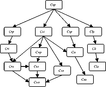
Fig.4 The Directed Acyclic Graph of Training Courses

Table I is a scores table of courses tests (partly). The data samples are collected from the previous test scores records of learners (280) in the distance education system. The score of courses has two distinct values (namely, { high , low }). When the score is more than 80, it is recorded as high ; when the score is less than 80, it is recorded as low .

TABLE I. T he S cores T able of C ourses T ests
ID	Courses No
	Cvp	Cvi	Cva	Crp	Cri	Cra	Cwp	Cwi	Cwa
1	high	high	low	high	low	low	high	high	low
2	high	high	high	high	high	low	high	high	low
3	high	low	low	high	low	low	low	low	low
4	low	high	high	high	low	low	low	high	low
5	high	low	high	high	high	high	low	low	low

P ( Crp = high | Cvp = low )

Numberof " Crp = high " and " Cvp = low "

Numberof " Cvp = low "

≈ 0.336.

Similarly,

P ( Crp = low | Cvp = low ) = 1 - P ( Crp = high | Cvp = low ) = 1 - 0.336 = 0.664.

Table II is a statistical table of tests scores (partly). It counts up the number of learners, who have the similar scores. Then, the simple probability and statistics method is used in computing the CPT.

TABLE II. T he S cores T able of C ourses T ests

Courses No                            Number of

Cvp Cvi Cva Crp Cri Cra Cwp Cwi Cwa Learners low low low low low low low low low 13 low low low low low low low low high 0 low low low low low low low high low 0 low low low low low low high low low 1 low low low low low high low low low 3 high high high high high high high high high 5 In Fig. 4, the node of Cvp has no parent, so the marginal posterior probabilities of Cvp may be estimated as follows:

The node of Cra has two parent nodes, Cvi and Cri . So, its conditional probabilities may be computed as follows:

P ( Cra = high | Cvi = high , Cri = high )

₌ Numberof " Cra = high "," Cvi = high " and " Cri = high " Numberof " Cvi = high " and " Cri = high "

= ⁵⁶ ≈ 0.747;

P ( Cra = low | Cvi = high , Cri = high ) = 1 - P ( Cra = high | Cvi = high , Cri = high ) = 1 - 0.747 = 0.253;

Numberof " Cvp = high "167

P ( Cvp = high ) =                        =    ≈ 0.596 ^.

TotleNumberof Learners 280

P ( Cra = high | Cvi = high , Cri = low )

₌ Numberof " Cra = high "," Cvi = high " and " Cri = low "

Similarly,

P ( Cvp = low ) = 1 - P ( Cvp = high ) = 1 - 0.596 = 0.404 .

The node of Crp has a parent node, Cvp . So, its conditional probabilities may be computed as follow:

P ( Crp = high | Cvp = high )

₌ Numberof " Crp = high " and " Cvp = high " Numberof " Cvp = high "

≈ 0.431.

Therefore,

Numberof " Cvi = high " and " Cri = low "

³⁶ ≈ 0.387;

P ( Cra = low | Cvi = high , Cri = low ) = 1 - P ( Cra = low | Cvi = high , Cri = low ) = 1 - 0.387 = 0.613;

P ( Cra = high | Cvi = low , Cri = high )

Numberof " Cra = high "," Cvi = low " and " Cri = high "

Numberof " Cvi = low " and " Cri = high "

²¹ ≈ 0.488;

P ( Crp = low | Cvp = high ) = 1 - P ( Crp = high | Cvp = high ) = 1 - 0.431 = 0.569.

In the same way,

P ( Cra = low | Cvi = low , Cri = high ) = 1 - P ( Cra = low | Cvi = low , Cri = high ) = 1 - 0.488 = 0.512;

P ( Cra = high | Cvi = low , Cri = low )

₌ Numberof " Cra = high "," Cvi = low " and " Cri = low " Numberof " Cvi = low " and " Cri = low "

= ¹³ ≈ 0.188;

P ( Cra = low | Cvi = low , Cri = low )

= 1 - P ( Cra = low | Cvi = low , Cri = low ) = 1 - 0.188 = 0.812.

Table III shows three parts of CPT as an illustration: A) the marginal posterior probabilities of Cvp , B) the conditional probabilities of Crp , C) the conditional probabilities of Cra . Then, the Bayesian networks can be used in classifying.

TABLE III. A I llustration of C onditional P robability T ables

a ) the marginal posterior probabilities of C VP

P( Cvp=high )	P( Cvp=low )
0.596	0.404

B) the marginal posterior probabilities of C RP

Cvp	P( Crp=high )	P( Crp=low )
high	0.431	0.569
low	0.336	0.664

C) the marginal posterior probabilities of C RA

Cvi	Cri	P( Cra=high )	P( Cra=low )
high	high	0.747	0.253
high	low	0.387	0.613
low	high	0.488	0.512
low	low	0.188	0.812

Table IV presents a sample set of training class-labeled tuples, D . The data are simplified for illustrative purposes. In reality, there are many more attributes to be considered. Note that each attribute is discrete-valued in this example. Continuous-valued attributes have been generalized.

The class label attribute, course_level, has three distinct values (namely, { high , middle , low }). Therefore, there are three distinct classes. Let class C L1 correspond to high, class C L2 correspond to middle, and class C L3 correspond to low.

Another class label attribute, student_value, has two distinct values (namely, { high , low }). Therefore, there are two distinct classes. Let class C V1 correspond to high and class C V2 correspond to low.

The target tuple is

X =( age = teenage , student = yes , investment = low , recency =5, frequency =4, monetary =2).

Take computing class label attribute, course_level , as an example. We need to maximize P(X|C Li )P(C Li ) , for i = 1, 2, 3.

The prior probabilities of each class can be computed based on the training tuples:

P(C_{L 1} ) = P(course_level=high)   = 2/15 = 0.133

P(C_{L 2} ) = P(course_level=middle) = 7/15 = 0.467

P(C L 3 ) = P(course_level=low)   = 6/15 = 0.400

In order to compute P(X|C Li ) , for i=1, 2, 3 , we compute the conditional probabilities of attributes, P(x_k|C_Li) , as follows:

P(age = teenage | course_level = high) = 1/2 = 0.500

P(age = teenage | course_level = middle) = 3/7 = 0.429

P(age = teenage | course_level = low) = 3/6 = 0.500

P(student = yes | course_level = high) = 1/2 = 0.500

P(student = yes | course_level = middle) = 5/7 = 0.714

P(student = yes | course_level = low) = 3/6 = 0.500

P(investment = low | course_level = high) = 1/2 = 0.500

P(investment = low | course_level = middle) = 4/7 = 0.571

P(investment = low | course_level = low) = 2/6 = 0.333

Using the above probabilities, we obtain

P(XIC L 1 ) = P(age = teenage | course_level = high) X

P(student = yes | course_level = high) X P(investment = low | course_level = high) = 0.500 X 0.500 X 0.500 = 0.125.

Similarly,

P(X\C L2 ) = 0.429 X 0.714 X 0.571 = 0.175

P(X\C l з ) = 0.500 X 0.500 X 0.333 = 0.083

To find the class, C Li , that maximizes P(X|C Li ) P(C Li ) , we compute

P(X\C l 1 ) P(C l 1 ) = 0.125 X 0.133 = 0.017

P(X\C l 2 ) P(C l 2 ) = 0.175 X 0.467 = 0.081

P(X\C l 3 ) P(C l 3 ) = 0.083 X 0.400 = 0.033

Therefore, the naïve Bayesian classifier predicts the class label course_level = middle for tuple X .

Accordingly, we can predict the class label student_value = high for tuple X .

• B.    System Experiment and Result Analysis

This experiment is based on the distance education system of vocational training. A training set, D , of class-labeled tuples randomly selected from the database of English learning information. First, the data preprocessing steps are applied to improve the accuracy and efficiency of the classification process, such as data cleaning, normalization and discretization.

TABLE IV. A S ample S et T able of T raining C lass - labled T uples

ID	Age	Student	Investment	Class: course_level	Recency	Frequency	Monetary	Class: student_value
1	youth	yes	low	middle	5	4	3	high
2	teenage	yes	low	middle	1	1	1	low
3	teenage	no	medium	low	2	3	1	low
4	youth	yes	low	middle	4	4	3	high
5	senior	no	high	middle	5	3	4	high
6	teenage	yes	low	high	3	5	5	low
7	youth	no	high	high	4	5	4	high
8	teenage	yes	low	middle	4	4	3	low
9	senior	yes	medium	low	1	2	1	low
10	teenage	yes	low	low	2	3	2	low
11	teenage	yes	medium	middle	5	5	2	high
12	senior	no	high	middle	4	4	3	low
13	youth	no	high	middle	3	3	2	low
14	teenage	yes	low	low	5	4	3	low
15	youth	no	medium	low	4	2	2	low

Next, the naïve Bayesian classifier produces a probability table by learning from the training set. The structure can be shown in Table V.

TABLE V. T he P robability T able of N aïve B ayesian C lassifier^*

ID

Class Label		Attribute
Name	Value	Name	Value
course_level	high
course_level	high	age	teenage
course_level	high	student	yes

Probability

0.133

0.500

0.500

Meaning

P(C L1 )

V. Conclusion

This study has built a learner classifier using the naïve Bayesian classification. It has exhibited high accuracy and objective. The classification rules can be used to support decision-making for achieving an excellent CRM for enterprises. And according to the dependencies between courses, Bayesian belief networks

^P(x1|CL1) are used to classify the learning resources and the

^P(x2|CL1) managers can also use the result of classification to draw

* The data in this table is from the previous subsection.

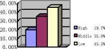
The classification results of 117 learners are illustrated in Fig. 5.

80.00%

60.00%

40.00%

20.00%

0.00%

a) Class: course_level

Fig.5 Classification result of 117 learners

□High 32.5% оLow 67.5%

up the suitable curriculum for learners. In general, Bayesian classification theories are useful analyses form to predict future data trends and make intelligent decision in distance education system. Moreover, with the thorough application of this DES, the result of classification and prediction will be increasingly accurate and useful. For future research, other types of business system can be considered to apply the Bayesian classifier model to deal with the resource allocation and customer

b) Class: student_value

management.