The Calibration Algorithm of a 3D Color Measurement System based on the Line Feature

Published Online October 2009 in MECS

The laser range finder (LRF) has been widely used together with a camera placed on a platform in 3D measurement [1] [2], robot motion planning [3], navigation [4] and collision avoidance [5], however, for these systems, there are still some difficult problems needing to be solved like:

• 1.    It’s difficult to measure the object far from the system;

• 2.    It’s difficult to measure the object outdoor;

• 3.    It’s difficult to measure a complicated scene;

• 4.    It’s difficult to measure an object with big size shape;

• 5.    It’s difficult to establish a colorful 3D model.

For an existed 3D measurement system to solve all the problems above; the price is very high and the arts and crafts are very complicated, which means it is not fit for the common applications. For common applications, a 3D color measurement system was established based on color camera, the 2D laser range finder with invisible stripe and platform in this paper to be used in SLAM (Simultaneous

Manuscript received Febuary 12, 2009; revised June 12, 2009; accepted August 13, 2009.

Localization and Mapping) problem study.

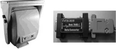
The sensors and corresponding data processing board are shown as Fig 1. As shown as Fig.1 (a), the camera is UC-800 (color 1024*768 pixels) made by UNIQ (America), and the corresponding data processing board is Meteor-II/Digital made by Matrox (America); as shown as Fig.1 (b), the LRF is LMS211 (360 spots, line scan, distance range [0,80]m, angle range[0,180] ° ) made by SICK (Germany), and the corresponding data board is CP132 made by Moxa (Taiwan); as shown as Fig1. (c), the platform is YA3050 made by Ya An(China), the corresponding switch is common switch form 485 protocol to 232 protocol.

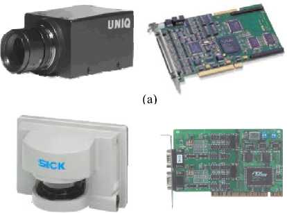
(b)

(c)

Fig.1. The sensors and the corresponding data processing board.

For the system, the critical problem is how to calibrate the 3 sensors precisely, which means to establish the homogenous transformation relationship of the data reference frames of the 3 kinds sensors. Because the LRF is more precise than the other sensors, we calibrate the system by calibrating the LRF with a platform and LRF with a camera. There is little reference about the calibration between LRF with invisible stripe and platform, because most 3D measurement applications [6] [7] uses the visible light spots, strip or pattern. But there are a few papers about the calibration between LRF and camera. Zhang and Pless presented a method for the extrinsic parameters calibration [8] based on the constraints between “views” of planar calibration patterns from a camera and LRF in 2004. But since the angle between the LRF’s slice plane and the checkerboard plane will affect the calibration errors, this method needs to put the checkerboard with a specific orientation, which is not easily established. Since the method is based on the data correspondence between the 3D range data and the 3D coordinates estimated by multi-views of the camera, the estimation errors of the 3D coordinates will affect the calibration result also. Bauermann proposed a “joint extrinsic calibration method” [9] based on the minimization of the Euclidean projection error of scene points in many frames captured at different view points. However, this method is only suitable for a device with the specific crane, and it establishes the correspondence between range and intensity data manually, which is also not easily established. Wasielewski and Strauss proposed a calibration method [10] mainly based on the constraints of projection of the line on the image and the intersection point of the line with the slice plane of the range finder in the world coordinate system. But the angle between the line and the slice plane of the LRF for different positions affects the calibration errors.

In order to solve all the problems presented above, a 3D measurement system was established as shown as Fig. 2. Firstly this paper analyzed 3 common geometrical features, and chose the line feature and designed rightangled triangular checkerboard. Secondly, we presented the calibration algorithms of 2D LRF, color camera and platform. Lastly, we described the experiments of the algorithms and the 3D color model reconstruction.

must be selected on a calibrated object and a set of constraints equations are established by associating the measurement data of the features of different sensors. The key issues include feature selection, derivation and solution of the constraint equations.

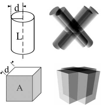
Three possible features: points, lines and faces, can be selected for the calibration. Consider the constraints on the extrinsic parameters when different features are used. First, if a point feature is used, the Position of the Camera or Platform (P-CP) is constrained on the surface of a sphere [2] [6] when the coordinates of the point with respect LRF coordinate frame is measured, provided that the measurement error is zero. When the measurement error is not zero, the camera is bounded to a spherical ring region. As shown in Fig. 3 (a), given the 3-D coordinates of the point measured by the laser range finder, the center O of the sphere is at the feature point and the radius d is the range measured by the LRF. For multiple feature points, P-CP is constrained to the intersection of the spherical surfaces. Second, consider the case when line features are used. As Fig. 3 (b) shows, P-CP is constrained in the inner space of the cylinder whose axis L is the line and radius is the measurement distance d of the LRF. For multiple line features, P-CP must be constrained in the intersection of the inner space of the cylinders. Finally, as shown in Fig. 3 (c), when a face feature is employed, P-CP is in the space between the measured plane A and the plane that is parallel to the face measured by the LRF and is apart from the face by the measured distance d . For multiple face features, the position of the camera is in the intersection of the spaces.

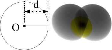
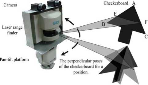
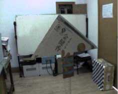
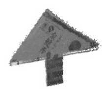
Fig. 2. The specific checkerboard is posed in the both views of the cameras and the laser range finder.

(b)

(c)

Fig. 3. Three possible features.

• II.    Features Analysis and Checkerboard Design

To calibrate the extrinsic parameters, a set of features

Obviously, point features lead to the smallest intersection space for constraining the camera’s position, and the constraints imposed by face features are the loosest. However, the light of the LRF is not visible, so it is impossible to use point features to establish the correspondence. Compared to face features, it is simpler and superior to establish correspondence between line features in the two different sensors. Lines can be easily detected by the camera. The intersection point of a line with the laser slice plane can also be easily detected by checking the changes in depth. Therefore, we adopted to use line features and design a checkerboard with rightangled triangular shape (Fig.2). The checkerboard is black so as to be easily detected in the image. At a given position and orientation of the checkerboard, we detect the projections of the two perpendicular edges of the camera and their intersections with the laser slice. Then, we establish the constraint equations by associating the intersection points with the projection. The use of a rightangled triangle is because of the fact that the intersection of the inner space of two cylinders is the smallest when they are perpendicular to each other. And for every different positions, the checkerboard is detected with two near perpendicular poses in a position as shown as the lower two checkerboards of Fig. 2. Therefore it is convenient to generate two pairs of perpendicular lines with great variety of rotation for every position.

• III.    Calibration Between LRF and Platform

• A.    Problems Defination

If t and Ф are the transition vector and the rotation vector and R is the corresponding rotation matrix, we could transform the coordinate P_L of the point P in LRF Coordinate Frame (LRFCF) to the coordinate in Original Platform Coordinate Frame (OPCF), which means the coordinate frame before rotation. Because the platform just rotates up and down in pitching direction, so we could define the origin of the axis Y of platform cross the origin of the LRF coordinate frame. So we can establish (1), (2) and (3) to reduce the parameters.

t = [0, ty, 0]T(1)

Ф = [Фx, Фy , Фz ]T(2)

PP = R X PL +1(3)

We can also estimate (4) and (5) to transform the coordinate of OPCF of point P from the coordinate in Rotation Platform Coordinate Frame (RPCF) of point P. Here Ф is the rotation vector, and the R is the w                                ,w corresponding rotation matrix. Then, from (1) to (5) we could establish (6).

Фw =[Фx, 0, 0]T(4)

P = Rw X Pp(5)

P = Rw X (R X PL +1)

Because the Ф w could obtain from the platform’s rotation control parameters, and P_L could be obtained from the laser range finder’s measurement. R_w is corresponding Ф w . It will be presented how to obtain the t and Ф corresponding R .

• B.    Constraint Equations

If py = [ p y ; , P 1 2 , L , py ; ] ^T and P2 = [ P 2 ; , P 2 2 , L , P2_n ] ^T are coordinates of OPCF from the measurements of the perpendicular edges by equation (6), when the platform rotates up and down, we can establish the estimates from three property of the points sequence.

• •    The linearity property:

Because the points sequence P Y ' and P 2 ' belong to the two line edges of the checkerboard, the errors of the line fitting for P Y ' or P 2 ' are very small. After the two points sequences were projected to 4 groups points in coordinate frame XZ and YZ, we could fit the 4 groups points to 4 lines. (A1ZX, B1ZX), (A1YZ, B1YZ), (A2ZX, B2ZX) and (A2YZ, B2YZ) are the coefficients of the 4 lines. And the errors of the 4 line fitting are V1ZX, V1YZ, V2ZX and V2YZ, which could presents the linearity property of PY and P 2 ' .

x = AYZXz + BYZX z = AYYZy + B1YZ x = A 2 ZXz + B 2 ZX z = A 2 YZy + B 2 YZ

• •    The Perpendicular Property:

  
  

From the coefficients of the 4 lines, we could also establish the direction vectors uY of PY and u 2 of P2'. From the coefficients, we also could obtain coordinate P1 and P2 of the two fitted lines. Then we could establish V to present the Perpendicular Property. Here “·” means

the scalar product of two vectors, and | …		| means the
absolute value.	1 ， 1 ] A 1 YZ
u Y = [ A Y ZX , ■		(9)
u 2 = [ A 2 zx ,	1 ， 1] A 2 YZ	(10)
PY = [ B Y ZX , -	B 1 YZ ,0] A 1 YZ	(11)
p 2 = [ B 2 ZX ,- V =| u Y	B 2 YZ ,0] A 2 YZ • u 21	(12) (13)

• The Coplanarity Property:

Because P Y and P 2 ' belong to the same plane of the checkerboard, the distance between two fitted lines could presented the coplanarity Property of P Y ' and P 2 ' . So we could use the (9), (10), (11) and (12) to establish (14).

Here “ X ” means the cross product of two vectors, and

“||......||” means the norm of the vector.

D = |( ulx u 2) •(p1 - p 2)1 || u1xu2 ||

• •    The Constrain Equation:

From the 3 properties, we can obtain the constrain equation (15). We solve the nonlinear optimization problem by using the Gauss Newton algorithm [11].

min ^ (V1ZX i² + V1YZ i² + V2ZX i² ■VZYZVI) ² ) (15) i

• C.    Calibration Algorithm

Step1: Set an initial value of Ф and t by a rough measurement or estimation.

Step2: Set the checkerboard nearer than other objects in front of the laser range finder, with movements of the platform, obtain the laser range finder’s data and the range of the platform’s pitching angle for different checkerboard’s position.

Step 3: Preprocess the laser range finder’s data, and establish the raw data sets for algorithm.

• (i ) Detect the scanning points on checkerboard by the distance discontinuity.

• (i i) Use the median filter to delete the error points.

• (i ii) After the line fitting to obtain the end points of the fitted line, we could obtain the intersection point sets between checkerboard and the scanning plane and the corresponding platform rolling angle sets.

Step 4: Transform the detected points coordinates to platform reference frame by (6) to get the

_______ points sets P and ^{P 2} . _________________ Step 5: Based on the P¹ and ^{P 2} ‘ , use (7), (8), (9), (10), (11), (12), (13) and (14) to establish the property functions. The constraint function was established by (15).

Step 6: By the Gauss Newton algorithm, the Φ and t could be obtained.

• IV.    Calibration Between LRF and Camera

• A. . Problem Definition

Fig. 1 shows a setup with a laser range finder and a stereo vision system for acquiring the environment information. We will use this setup in the experiments. It is necessary to find the homogeneous transformation between every camera and the LRF in order to fuse the measuring of the camera and the LRF. Two coordinate frames, namely the camera coordinate frame (CCS) and the laser range finder coordinate frame (LRFCS), have been set up to represent the measurements with respect to the respective sensors. The objective here is to develop an algorithm for calibrating the orientation vector

Ф 0 , 0 y , 0 z )and the translation vector t ( t x , t y , t z ) of the camera with respect to the laser range finder. Let R be the rotation matrix corresponding to the orientation angles Ф . Denote the coordinates of a point p with respect to the CCS and LRFCS by p _C and p _L , respectively. The coordinates are related as follows.

P C = Rp L ⁺ t                  ⁽¹⁶⁾

The raw measurements of LRF are expressed in the polar coordinates on the slice plane as ( p , 0 ), where p represents the distance and 0 is the rotation angle. Then the coordinates p_L is given by (17):

p L = [ p l cos 0 , p l sin 0 , 0 ] ^{T         (17)}

• B.    Constraint Equations:

As Fig 1 shows, it denotes the two perpendicular edges of the checkerboard by lines AB and AC , respectively, and their intersections with the laser slice plane by points E and F , respectively. In the calibration, we use two kinds of measurement data obtained at different poses of the checkerboard. One kind of data is the projections of the two perpendicular lines ab and ac on the image planes, and the other is the measurements of the intersection points E _L and F _L in LRFCS.

Assume that the camera is a pinhole camera. Given the distortion coefficients k ( k 1 , k 2 , k 3 , k 4 , k 5 ) and the intrinsic parameter matrix K , a point E _C ( x_E , y_E , z_E ) in the camera coordinate frame can be projected onto the point e ( x, y_e ) on the image plane by using (18) and (19) ([12] and [13]), where ( x d ,, y_d ,1) is the normalized coordinate including lens distortion in CCS.

(1 + k 1) r2 + k 2 r4 + k 5 r 6)

• ² k 3 xy + k ₄ ⁽ r ² + 2 x ²⁾ k ₃( r ² + 2 y ²) + 2 k ₄ xy

  x_d     x

  y_d     y

  
  

x

x = — zE y = yk zE

r = 7 x2 + y2

"е 1      ^ xd 1

y_e = K y d

1                1

As Fig. 1 shows, on the image plane, the projection ab of edge AB can be detected. E _L is the point measured by the LRF. e is the calculated projection of point E _L by using (16) (17) (18) and (19). Then the distance d ( e , ab ) from the point e to the line ab can be calculated by using (20) [14].

uur uur d (e, ab) =       ab                    (20)

||ab|| where “×” is the cross product of two vectors, ab is the vector from point a to point b , eb is the vector from point e to point b and ||…|| is the norm of the vector.

Similarly, for the edge AC and intersection point F , we can also calculate the distance d ( f ， ac ) from the calculated projection f of the point F to the projection ac of edge AC on the image plane. For different orientations and positions of the checkerboard, we obtain different distances. Introduce an index i to represent the distances at different orientations and positions. The calibration problem of the extrinsic parameters can be formulized as a problem of finding the optimal solution of the translation vector t and orientation angles Φ that minimize the sum of the distances as shown as (21).

min      d ( e , ab ) ＋ d ( f , ac ) ²          (21)

I i i i                          i ii

Where the index i represents the i -th position and orientation of the checkerboard. We solve the nonlinear optimization problem by using the Gauss Newton algorithm [11]. The initial parameters used are values obtained by a rough measurement for the device. The initial parameters can also be obtained by the closed form solution proposed in [8].

• C.    Calibration Algorithm:

Step1: Set an initial value of Φ and t by a rough measurement or estimation.

Step2: For different checkerboard position, detect the two point sets and project the points to image coordinate.

• (i)    Detect the points in checkerboard based on the distance discontinuity of all scanning points.

• (ii)    Use median filter to delete the error points from the detected points.

• (iii)    Use line fitting and obtain the intersection points of the scan plane and the checker board’s edge line from the fitting line’s end points.

• (iv)    Use (16), (17) and (18) to transform the points from the laser range finder coordinates to camera coordinates.

• (v)    Use (19) to transform the points from camera coordinates to the image coordinates.

Step3: Detect the projections of the perpendicular edges of checkerboard on the image plane and calculate their coordination on the image plane.

Step4: Based on the checkerboard’s vertexes coordinates in image reference frame and the laser range finder reference frame, use (20) and (21) we could establish the constrain functions.

Step5: By the Gauss Newton algorithm, the Φ and t could be obtained.

• V. Experimental Results

  After we proved the effectiveness by these experiments using these two algorithms, we presented the experiment of 3D color reconstruction of a complicated scene by the calibration results to show the system’s effectiveness. We also conducted experiments on the setup shown in Fig. 1. On a pan-tilt platform, two UNIQ UC-800 cameras with 1024*768 pixels are mounted with a SICK LMS221-30206 LRF, which can provide 100 degrees and maximum 80(m) measurements with the accuracy of ± 50(mm).

• A. . The Experimental Results of LRF and Platform

  
  
  
  
  
  

(a) the image of           (b) projection of X- checkerboard                  Z Frame

^i;^-s''

(c) projection of

(d) projection of

Y-Z Frame

X-Y Frame

(e) 3D color reconstruction result

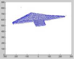
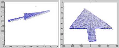
Fig.4. 3D reconstruction of the checkerboard.

As Fig.4 shows, the measurement of the checkerboard was reconstructed to present the precision of calibration results between LRF and camera. The real sizes of the checkerboard’s edges are 315mm, 380mm and 491mm. From the measurement of reconstruction by MATLAB software, the sizes of 3D reconstruction model’s edges are 300.3633mm, 373.4127mm and 496.2991mm. Then the mean of the errors is 8.8410mm, which is better than the accuracy of LRF. So the calibration is effective.

• B.    The Experimental Results of LRF and Camera

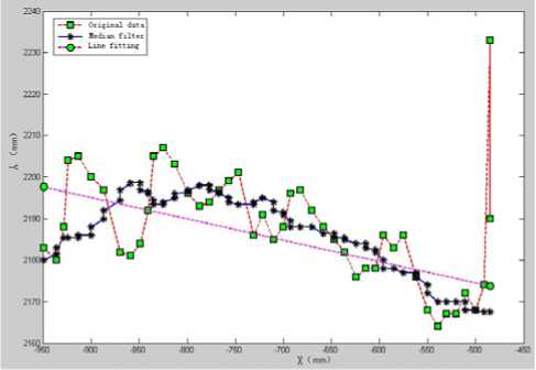
After detecting the point sets on the checkerboard, we found that there are lot’s of error measure points near the checkerboard’s edges, because the laser range finder have the mixture pixel effect. Fig. 5 shows the mixture pixel effect and the preprocessing results of the original data to remove the error points. Fig. 5 (a) shows the real preprocessing results of the original data. The points of Fig. 5 (a) show the detected points by discontinuity and selecting the points near from the laser range finder, and the line shows the line fitting results. The end points of the line correspond with the intersection points between the scanning plane and the checkerboard. Fig. 5 (b) shows the two main steps of the preprocessor, one is median filter as shown as the cross points, the other is line fitting, as shown as the round points, and the square points shows the original points. Form original points of the experiment we could find that it’s difficult to get the real intersection points between the scanning plane and the checkerboard plane. From the experimental results, we could find that the median filter could effectively remove the “jump points”, and the line fitting could effectively decrease the measurement error and noise effect.

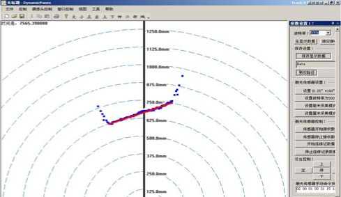
(a) the interface of data collection software

(b) the preprocessor of the original data

Fig.5. The original data collection and the preprocessor

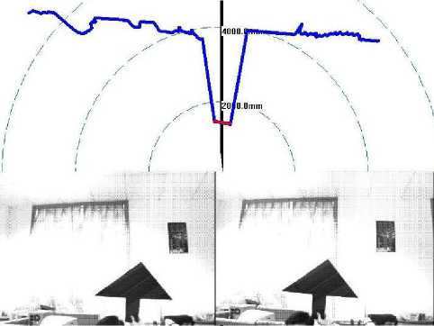
Fig.6. The raw data obtained by the LRF and two cameras.

We employed the proposed algorithm to calibrate the homogeneous transformation between the LRF and each of the cameras. In the experiments, the checkerboard was placed closer to the LRF than the background to easily distinguish the checkerboard from the background. 20 positions were used to calibrate the extrinsic parameters. Fig.6 shows the raw data obtained by the LRF and the cameras for a pose of the checkerboard. The upper image of Fig.5 shows the LRF’s measurements. In order to precisely detect the intersection points’ coordinate, the median filter and the least square line fitting were used to process the detected measurement data of the LRF. As the upper image of Fig. 6 shows, the bottom line of the measurements is the result of the line fitting. The edges of the checkerboard on the bottom images in Fig. 6were detected manually.

To demonstrate superior performance of our method over the method in [8], we projected the measurements of the LRF onto the images of the two cameras using the extrinsic parameters calibrated by both methods. The results are shown in Fig.7. The upper solid lines represent the projections of the LRF measurement using the parameters calibrated by our method, and the lower dotted lines denote those obtained by the method in [8]. Obviously, the projected points obtained by our method more fit the scene in the two images. Therefore, it is possible to conclude that our method can calibrate the extrinsic parameters more accurately.

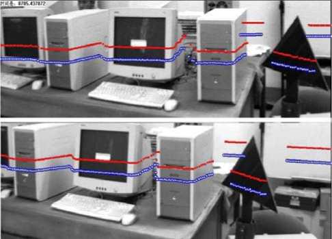
Fig.7. Projections of the LRF measurements onto the image planes of the cameras using the parameters calibrated by our method and the method in [8]. (Upper image: the left camera, lower image: the right camera)

• C.    The Experimental Results of 3D Color Reconstruction

After the calibrations of the system, we measured a complicated scene indoor. Because the sensors could scan the scene and objects by scanning movement, the system could measure bigger objects and more complicated scenes, which could be more far from sensors than lot’s exist measurement system. Fig. 8 shows 3D color reconstruction of point clouds for the complicated scene indoors, and the Fig.8 (b) shows the 3 shot screen of the 3D reconstruction model from 3 different views. From the reconstruction result, we could find that the measurement system could reconstruct the scene true to nature and in detail, such as the paper on the table. Fig. 8 shows the other reconstruction results of the complex scene indoors.

• VI. Conclusion

A novel 3D color measurement system was presented in this paper for SLAM problem. After three common features were compared with each other, the calibration algorithms for LRF, camera and platform were presented based on the line feature. The real data experimental results of the algorithms and the 3D color reconstruction model show the effectiveness and the efficient of algorithms and the system.

Acknowledgment

The work really thanks the Prof. Yunhui Liu of Hongkong Chinese University. Without his kindly help and the direction, the work and the project could not be completed.

• [2]    L. D. Reid, “Projective Calibration of A Laser-stripe Range Finder,” Image and Vision Computing, vol.14, no.9, pp.659-666, October 1996.

• [3]    H. Baltzakis, A. Argyros, and P. Trahanias, “Fusion of Laser and Visual Data for Robot Motion Planning and Collision Avoidance,” International Journal of Machine Vision and Applications, vol.15, no. 2, pp. 92-100, 2003.

• [4]    T. Hong, R. Bostelman, and R. Madhavan, “Obstacle Detection Using A TOF Range Camera for Indoor AGV,” Navigation, PerMIS 2004, Gaithersburg, MD, June 2004.

• [5]    I. Bauermann, E. Steinbach, “Joint Calibration of A Range and Visual Sensor for the Acquisition of RGBZ Concentric Mosaics”, VMV2005, November 2005.

• [6]    J. Forest, J. Salvi, "A Review of Laser Scanning Threedimensional Digitizers,” In IEEE/RSJ International Conference on Intelligent Robots and System. EPFL Lausanne, Switzerland, vol.1, pp. 73-78, 2002.

• [7]    J. Davis and X. Chen, “A Laser Range Scanner Designed for Minimum Calibration Complexity,” In 2001 IEEE Third International Conference on 3D Digital Imaging and Modeling, Canada, pp. 91-98, 2001.

• [8]    Q. L. Zhang, R. Pless. Extrinsic calibration of a camera and laser range finder (improves camera calibration). In 2004 IEEE/RSJ International Conference on Intelligent Robots and systems, Sendai, Japan, 2004, 2301~2306.

• [9]    I. Bauermann, E. Steinbach. Joint calibration of a range and visual sensor for the acquisition of RGBZ concentric mosaics. VMV2005, November 2005.

• [10]    S. Wasielewski, and O. Strauss. Calibration of a multisensor system laser rangefinder/camera. Proceedings of the Intelligent Vehicles '95 Symposium, Sep. 25-Sep. 26, 1995, Detroit, USA Sponsored by IEEE Industrial Electronics Society, 1995, 472~477.

• [11]    J. Stoer, and R. Burlisch. Introduction to Numerical Analysis. Springer Verlag New York Inc, 1980.

• [12]    G. Q. Wei, and S. D. Ma, “Implicit and Explicit Camera Calibration: Theory and Experiments,” IEEE Transaction Pattern Analysis and Machine Intelligence, 16 (5): 169-180, 1994.

• [13]    G. Q. Wei, and S. D. Ma, “Implicit and Explicit Camera Calibration: Theory and Experiments,” IEEE Transaction Pattern Analysis and Machine Intelligence, 16 (5): 169-180, 1994.

• [14]    H. Wang, “The Calculation of the Distance between Beeline and dot,” Journal of Shangluo Teachers College of China, vol. 19, no.2, pp.16-19, 121, June 2005.

Li Ganhua (Xi’an, China, June 10, 1977 ), Ph. D (2007). He get the Ph. D in National University of Defense Technology, which is in the Changsha city, Hunan province of China. His major field is information technology, image process, data fuse, target recognition.

G.H. Li is the senior engineer in Xi’an satellite control center. He has been the main actor of more than 10 important project witch are supported by military foundation, 863 high technology foundation and the country predict foundation. He is interest in the 3D reconstruction technology, target recognition and the image process.