The comparison of efficiency of the population for-mation approaches in the dynamic multi-objective optimization problems

Multicriteria optimization in a non-stationary environment (dynamic multi-objective optimization, DMOO) is a complex and currently insufficiently studied class of optimization problems. In such problems, objective functions, their parameters, and restrictions imposed on the search area can change over time [1]. At the same time, the objective functions in this case are a “black box”, therefore, the form of the objective functions and their properties remain unknown, and there is also no possibility of calculating derivatives, which greatly complicates the choice of an appropriate method for solving this class problems. At the moment, a number of approaches to solving problems have been proposed, however, these approaches can provide a successful solution of a problem only if it has a strictly defined form, so it is necessary to continue researching approaches for solving this type of problems.

Multicriteria non-stationary optimization

The DMOO problem can be represented as a set of two other optimization problems: a multiobjective optimization (MOO) problem and a dynamic optimization (DO) optimization problem in a non-stationary environment.

A feature of the multicriteria optimization problem is the presence of two or more objective functions that must be optimized simultaneously. Thus, when finding a solution to the problem, it is necessary to take into account the values of all objective functions. Formally, the problem of multiobjective optimization can be represented as

{ f ₁( x ), f ₂( x ),..., f_k ( x )} → min ,                                     (1)

x where fi is a set of optimizable functions; i ∈ [1, k]; k is a number of objective functions; x is a decision vector from the allowable region S.

As mentioned above, the objective functions in most practical problems conflict with each other, that is there is rarely a solution that would be optimal immediately for all target functions. Often it is necessary to choose a compromise solution, in which the values of the objective functions are acceptable in a certain sense, using a set that is Pareto optimal (Pareto set, PS) [2].

Many applied optimization problems are in conditions that change over time. Such problems are called optimization problems in a non-stationary environment or time-dependent optimization problems. A feature of DO problems is that search space of a problem and landscape of the objective function change over time, and at the same time, the optimal solution to the problem also changes [3].

In many publications considering DO, it is proposed to use evolutionary algorithms (EA) to find a solution to this type of problem. The EA class is a good tool for solving DOs because these algorithms are inspired by natural systems that are constantly under the influence of changing factors. EAs operate with a population of solutions, so in the case when the optimal solution to the problem changes, one of the available solutions can be quite close to the optimal one.

The DO task can be formally defined as follows [3]:

f(x,a(t)) →min , (2) x where f - objective function; x - solution vector from the search space; a(t) - vector of some timevarying objective function parameters; t e [0, T] - time interval in which the problem is considered.

In practical problems, the vector a ( t ) can represent the parameters of the external environment (such as, for example, temperature, available resources, etc.) that affect the objective function. In artificially generated test problems, for example, in problems with moving extremum areas - depressions, this can be a parameter of their depth, width and location. The vector a ( t ) can also include other variable parameters, for example, the number of variables of the objective function [4].

Most of the existing works on DO consider this problem as a sequence of problems on a discrete time interval t e {0,^, T }:

{ f ( x , a (1)) → min, f ( x , a (2)) → m i n,..., f ( x , a ( T )) → m i n} . xx   x

The definition of a DMOO problem can be represented as follows [4]:

{ f ₁( x , a ( t )), f ₂( x , a ( t )),..., f_k ( x , a ( t ))} → min . x

The complexity of multicriteria optimization in a non-stationary environment lies in the fact that along with a change in the problem, a change in the Pareto front (PF) occurs.

Publications on DMOO provide different ways of classifying such problems, depending on the type of change [4]:

• -    classification based on the rate of change. With an increase in the rate of change, the allowable time for the algorithm to adapt to emerging changes decreases, which complicates the problem;

• -    classification based on the degree of change. Changes can be major or minor. In case of minor changes, it is possible to use information obtained from the previous state;

• -    classification based on the predictability of changes. Changes can be regular (cyclic) and, as a result, predictable, or random (acyclic);

• -    classification based on the variability of PF and PS. This classification option includes 4 types of problems: the optimal PS changes, the optimal PF does not change; both the optimal PF and the optimal PS change; the optimal PS does not change, the optimal PF does not change; both the optimal PS and the optimal PF do not change. In the latter case, for example, only local extrema can change.

There are two ways taking into account the changes occurring in the task [5]:

• 1.    Consider every change as a new optimization problem that needs to be solved from scratch.

• 2.    Use information from the previous solution step to speed up the optimization process after the change.

However, the first approach is not always suitable due to time limits. In the second case, the algorithm must be able to adapt to changes, that is there must be sufficient diversity in the solutions used so that the algorithm can respond flexibly to changes.

In the works devoted to DMOO, approaches to solving such problems based on existing EAs are considered:

• -    approaches based on the introduction of mechanisms in EA that contribute to an increase in diversity (diversity based [6,7]);

• -    approaches based on prediction of changes in the problem (prediction based [8; 9]);

• -    approaches based on the use of information about the previous state in the problem when searching for a solution in the current state (memory based [10; 11]);

• -    approaches based on the use of several populations evolving in parallel to each other and exchanging information (multi-population based [12; 13]).

Application of EA for solving DMOO problems is currently insufficiently studied, while the use of EA for solving MO problems is much more developed - for this class of problems there are a number of widely used methods based on EA, such as, for example, NSGA-2 and SPEA2, which allow to approximate PF with high accuracy. Therefore, it makes sense to use already existing methods in the formation of approaches to solving DMOO problems.

Algorithm NSGA-2

(Non-dominated Sorting Genetic Algorithm) is one of the most well-known algorithms for solving the multiobjective optimization problem. Figure 1 schematically shows the principle of operation of two decision sorting mechanisms used in NSGA-2: non-dominated decision sorting and crowding distance sorting [14].

The sorting of non-dominated solutions is as follows. The total population R t consists of the population of parents R t and the population of their descendants Q t , its size is 2N , where N is the size of the population. Further, the solutions in the set R t are sorted as follows: the subset F 1 includes all nondominated solutions (solutions for which there are no dominant solutions in the population) - this is called the first non-dominated front; the subset F 2 includes solutions that are non-dominated within the set { R t / F 1 } (the set R t , excluding the subset F 1 ), this is called the second non-dominated front, etc.

Next, a new population P t +1 is formed: subsets of non-dominated fronts are added in turn, starting from the first, to the population Pt + 1 until the size of the subset of the next non-dominated front does not exceed the available size of P t +1 . In this case, solutions are sorted according to their degree of crowding: for solution i , the distance to neighboring solutions is calculated (Fig. 2). Thus, a variety of solutions enter the population.

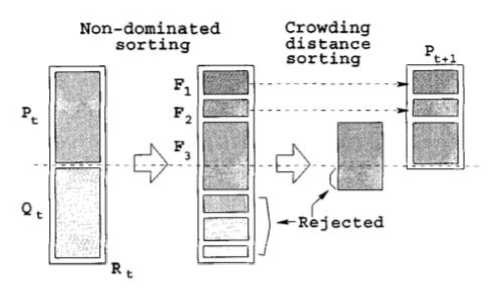
Рис. 1. Механизмы сортировки в NSGA-2 [14]

Fig.1. Procedure of sorting a population in NSGA-2 [14]

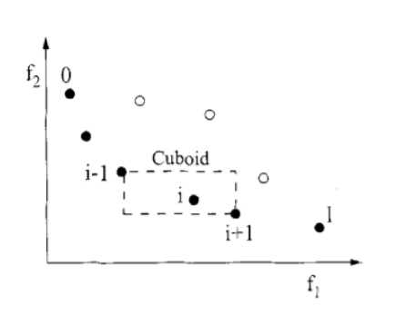
Рис. 2. Сортировка по степени скученности в NSGA-2 [14]

Fig. 2. Crowding distance sorting in NSGA-2 [14]

После чего к новой популяции P t+1 применяются операторы селекции, рекомбинации и мутации. After that, selection, recombination and mutation operators are applied to the new population P t+1 .

Algorithm SPEA2

The SPEA2 algorithm (Strength Pareto Evolutionary Algorithm) is also one of the most popular multiobjective optimization algorithms. One of its features is that, along with a population of solutions, the algorithm uses an archive of non-dominated solutions (external set) [15]. To maintain a given number of individuals stored in the archive, they are clustered according to the degree of remoteness from each other, as a result of which only a representative of the cluster remains in the archive. The use of an archive of solutions allows the algorithm to better approximate the Pareto front in comparison with other algorithms.

Another feature of the algorithm is the calculation of the suitability of individuals. To begin with, each individual i in the population P t and in the external set P t^* is assigned the value of "force" S , which is the number of individuals who dominate the considered individual [15]:

S ( j ) = { j | J ^e P t + P t * л i^j }|

where means Pareto dominance. However, a high "force" value does not guarantee that the solution is close enough to the Pareto frontier. Therefore, further the value R is calculated for each individual, which is the sum of the values of the "forces" of individuals dominating over the one under consideration,

R ( i ) = Z    S ( j ).

J ^e P t ⁺ P t *, j^

Thus, the value R = 0 corresponds to a non-dominated solution (Fig. 3):

4        0

У___• nondominated

• •  ■—• dominated

0 о о 5 о о 12

О о

оо

Рис. 3. Ранжирование решений в SPEA2 [15]

Fig. 3. Ranking of solutions in SPEA2 [15]

The resulting fitness F(i) of an individual is calculated as the reciprocal of R :

F (i) = —1—.(7)

1 + R (i)

After that, tournament selection, recombination, and mutation operators are applied to the solution population.

Description of numerical experiments

When using the multiobjective optimization algorithm, the problem of non-stationary optimization at each time t is considered as a separate optimization problem. There are two options for the formation of the initial population during the transition from one point in time to the next one:

• 1.    Initialize the population randomly, restart the algorithm.

• 2.    Use the population of solutions obtained at the previous time.

• 3.    Use a population of solutions, one part of which was obtained at the previous time, and the other was randomly initialized.

It is necessary to check whether there is a difference in the accuracy of the obtained solutions and the speed of convergence between these three methods. Further, these methods will be considered using the NSGA-2 and SPEA2 multiobjective optimization algorithms as an example.

As test problems of multicriteria non-stationary optimization, we took a set of CEC2018 Dynamic Multi-objective Optimization Benchmark Problems, which includes tasks of various types. Table 1 presents the characteristics of the tasks, given in [16].

Table 1

Characteristics of test problems

Problem	Quantity	Type of change	Notes
DF1	2	Mixed convexity-concavity, change in the position of optima	Non-stationary PF and PS
DF2	2	Changing positions of optima	Stationary convex PF, non-stationary PS
DF3	2	Mixed convexity-concavity, change in the relationship between variables, change in the position of optima	Non-stationary PF and PS
DF4	2	Changing the relationship between variables, changing the values of the boundaries of PS and PF	Non-stationary PF and PS

DF5	2	Changing the number of concave and convex areas, changing the position of optima	Non-stationary PF and PS
DF6	2	Mixed convexity-concavity, multimodality, change in the position of optima	Non-stationary PF and PS
DF7	2	Changing the range of PF and the position of optima	Non-stationary PF and PS, stationary centroid PS, convex PF
DF8	2	Mixed convexity-concavity, change in the position of optima, PS points have a regular distribution structure	Non-stationary PF and PS, stationary centroids PS, dependence between variables
DF9	2	Change in the number of unconnected PF segments and the position of optima	Non-stationary PC and PS, dependence between variables
DF10	3	Mixed convexity-concavity, change in the position of optima	Non-stationary PC and PS, dependence between variables
DF11	3	Changing the size of the PF region, the range of the PF, and the position of the optima	Non-stationary PF and PS, concave PF, dependence between variables
DF13	3	Change in the number of unconnected PF segments, change in the position of optima	Non-stationary PF and PS, PF can be a continuous concave or convex segment, or several disconnected segments
DF14	3	Change in the number of concave and convex regions, change in the position of the optima	Non-stationary PC and PS, dependence between variables

The type of tasks changes depending on the value of the parameter t . The moment of time t in the test problems from this set is determined as follows:

1 т t =

п LT t where nt – intensity of change; τ = i∙n; i – problem iteration number; n – number of iterations of the optimization algorithm; τt – rate of change.

To assess the accuracy of the obtained solutions for multicriteria optimization problems, the IGD (Inverted Generational Distance) measure is used, which shows the degree of difference between the initial PF P and the found PF P* [17]. For problems of non-stationary multicriteria optimization, the average MIGD measure is used:

TT^nP t ⁱ

MIGD = 7 EIGD ( P*, ^p t ) = 7 EE — ,                 (9)

T t=1                     T t=1 i=1 nPt where nPt = |Pt|; dti – Euclidean distance between i element of Pt and the nearest to it element Pt*; T – number of problem iterations.

The Hypervolume measure is also used, which shows the degree of remoteness of the front from some worst reference point, which is set manually [18]. For problems of non-stationary multicriteria optimization, the averaged measure MHV is also used:

T

MHV = 7 E HV t ( P t *),                           (10)

T t = 1

where HV t – hypervolume operator. In [16], it is proposed to specify the worst point as ( z 1 + 0,5, z 2 + 0,5, …, z m + 0,5), where z j –the maximum value of the j objective function in the initial PF at time t; m is the number of target functions.

When carrying out numerical experiments, the following values of test problem parameters were used:

• -    intensity of changes n τ is 10;

• -    the number of iterations of the problem T is 30;

• -    the number of problem variables is 10.

Numerical experiments were performed using two different values of rate of change τ t : 10 (fast changes) and 30 (slow changes) in order to check whether no restart gives a better result with slower changes in the problem.

Also, for the NSGA-2 and SPEA2 algorithms, the population size was set to 50 and the number of generations to 30. Each test problem was solved 20 times, the results were averaged.

Results

Table 2 shows the average IGD metrics for each test task at slow and fast rates of change and using the NSGA-2 and SPEA2 algorithms. The results are compared with each other when using a restart in the algorithm (population initialization is random), without using a restart (using a population obtained at the previous time point) and with a 50% restart (one half of the population is initialized randomly, and the other half is randomly selected solutions from population obtained at the previous point in time). Table 3 shows the average values of the HV metric.

The results were processed using the Mann-Whitney statistical test. The statistically best values of the metrics are highlighted in green (within the framework of the algorithm used); highlighting multiple columns with color means that the differences between them are not statistically significant.

IGD metric values depending on different population initialization with slow and fast changes for NSGA-2 and SPEA2 algorithms

Table 2

Slow change
Problem	NSGA-2			SPEA2
	With restart	Without restart	Restart 50 %	With restart	Without restart	Restart 50 %
DF1	0.16626	0.05562	0.06047	0.35837	0.19831	0.14915
DF2	0.4249	0.39807	0.34611	0.64654	0.51556	0.43324
DF3	1.07812	0.46373	0.63423	1.48503	0.29893	0.31623
DF4	1.70829	0.2219	0.23465	3.21155	0.31159	0.30098
DF5	3.27418	2.86193	3.17044	3.54135	3.44858	3.16089
DF6	5.82266	4.37637	3.9914	7.65581	10.31912	6.58776
DF7	2.88988	0.21077	0.29967	0.57322	0.14004	0.16273
DF8	0.4861	0.24668	0.46732	0.36439	0.06035	0.07962
DF9	1.11271	1.00767	0.87972	1.00105	0.77221	0.35849
DF10	0.63374	0.20805	0.28913	0.80103	0.16978	0.2983
DF11	1.33799	1.20587	1.21676	1.52398	1.248	1.26458
DF13	1.14789	0.82343	0.92381	1.99445	0.92517	0.59001
DF14	1.96974	2.15505	2.46098	0.86397	024935	0.24797
Fast change
Problem	NSGA-2			SPEA2
	With restart	Without restart	Restart 50 %	With restart	Without restart	Restart 50 %
DF1	0.15418	0.37973	0.1188	0.34685	0.67789	0.23528
DF2	0.43164	0.7622	0.3886	0.67347	0.98689	0.53114
DF3	0.99878	0.8379	0.91423	1.4139	0.65215	0.59109
DF4	1.75676	0.19023	0.20557	3.34937	0.30802	0.31553
DF5	5.48928	5.47719	5.51248	5.78571	6.27579	6.03813
DF6	5.83975	15.35728	7.55838	7.94478	19.964	7.73518
DF7	3.71561	0.41029	0.66258	0.66013	1.09603	0.562
DF8	0.4835	0.25431	0.46186	0.35465	0.07659	0.08844
DF9	1.06701	1.91676	1.07585	0.99857	2.52754	0.94053

DF10	0.55375	0.19654	0.24747	0.6755	0.15305	0.23408
DF11	1.31739	1.21583	1.21464	1.51375	1.25063	1.2498
DF13	1.11659	1.03303	0.91568	2.01859	3.41013	1.16391
DF14	1.96235	2.78436	2.68979	0.85173	0.51699	0.4661

Table 3

HV Metric Values Depending on Different Population Initialization with slow and fast changes for NSGA-2 and SPEA2 algorithms

Slow change
Problem	NSGA-2			SPEA2
	With restart	Without restart	Restart 50 %	With restart	Without restart	Restart 50 %
DF1	1.32092	1.54591	1.53165	0.96699	1.24592	1.34441
DF2	1.15173	1.14765	1.2953	0.7926	0.96943	1.11871
DF3	0.37984	0.84905	0.72257	0.14168	1.09988	1.07317
DF4	4.05769	7.6282	7.58849	1.28999	7.3678	7.36317
DF5	137.27398	139.51692	138.1649	111.54741	113.28194	113.31316
DF6	0.18186	0.60413	0.61594	0.0376	0.21177	0.20861
DF7	0.60904	2.95476	2.64463	2.05972	3.08956	3.00454
DF8	0.82234	1.49508	0.94826	1.03271	1.73879	1.6861
DF9	0.20507	0.39313	0.37082	0.3858	0.88429	1.05993
DF10	1.37764	2.56913	2.39078	1.10203	2.6405	2.32359
DF11	0.30304	0.50691	0.49764	0.07836	0.44429	0.41238
DF13	7.55833	10.14608	8.68482	1.08663	3.19273	4.40662
DF14	0.0873	0.06332	0.09364	0.1999	0.75084	0.73419
Fast change
Problem	NSGA-2			SPEA2
	With restart	Without restart	Restart 50 %	With restart	Without restart	Restart 50 %
DF1	1.38279	1.07766	1.45141	1.02725	0.80304	1.22049
DF2	1.14435	0.70886	1.20913	0.75946	0.5301	0.95102
DF3	0.43748	0.66908	0.60571	0.19885	0.19885	0.77118
DF4	3.37641	6.5282	6.4919	0.94274	6.24129	6.20666
DF5	294.16315	295.48085	295.87608	238.39456	236.6676	240.46001
DF6	0.17802	0.29026	0.28404	0.03593	0.07157	0.12937
DF7	0.97366	3.33281	2.84268	2.64918	3.08993	3.28456
DF8	0.85182	1.51224	0.9437	1.0689	1.74353	1.70175
DF9	0.24943	0.121	0.2484	0.40496	0.17604	0.45905
DF10	1.72413	2.72373	2.60652	1.4608	2.79819	2.55707
DF11	0.33402	0.53781	0.53404	0.08475	0.47655	0.45826
DF13	7.66373	9.09398	8.21799	1.11795	1.1479	2.48469
DF14	0.0907	0.04726	0.08153	0.2078	0.45549	0.44884

From the results presented in the table, it can be seen that in the case of slow changes in solving most test problems, the use of the population obtained in the previous step is the most effective. However, in the case of fast changes, you can see an increase in the number of problems for which the use of a restart (either full or 50%) is most effective. This is due to the fact that with fast changes, the state of the problem at the previous step differs from the state at the current step to a greater extent compared to slow changes.

Figure 4 shows diagrams of the rank values assigned to the metric value for each of the six variants of the algorithm and summarized over all test problems. For the best value of the metric, the highest rank was assigned. To ensure the reliability of the ranking, a test of the significance of differences in the results was carried out using the criterion Mann-Whitney: the test was applied to a pair of closely ranked results. If the differences are insignificant, then these two results were assigned the average value of their ranks. It can be seen that there is no significant difference between the use of the NSGA-2 algorithm and

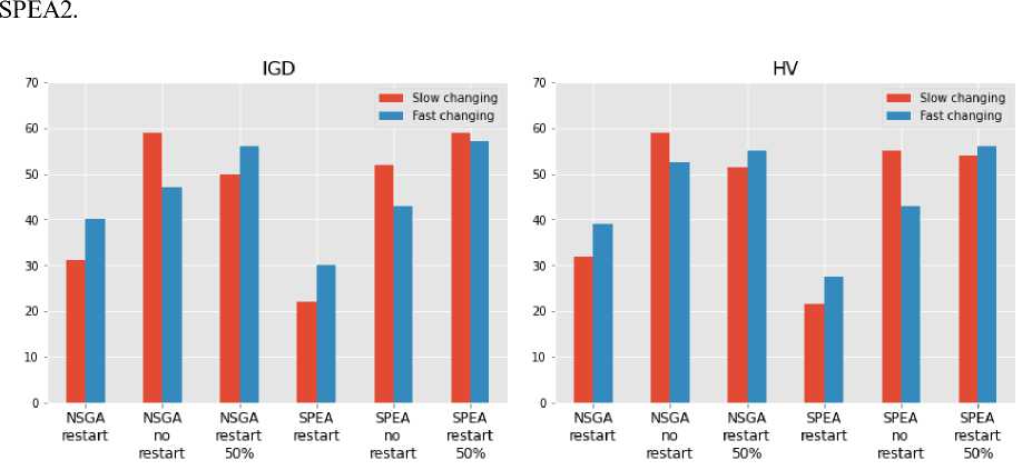
Рис. 4. Диаграммы значений суммарных рангов использованных алгоритмов

Fig. 4. Diagrams of the ranks values of the algorithms

Figures 5 and 6, using the example of two test problems, show graphs of the change in the values of the metrics IGD and HV at each iteration of the NSGA-2 algorithm with slow (top) and fast (bottom) changes. You can see that every 30 iterations of the algorithm there is a abrupt jump in the values of the metrics, at this moment a change in the problem happens.

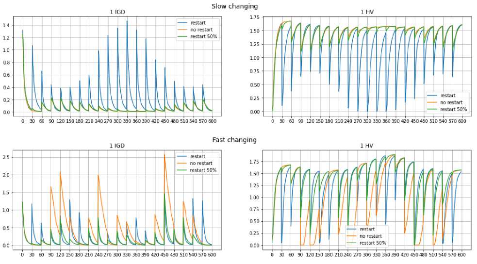
Рис. 5. Изменение значений метрик на примере задачи DF1 при медленных и быстрых изменениях

Fig. 5. Changing values of IGD and HV metrics in DF1 problem in the cases of slow and fast changes

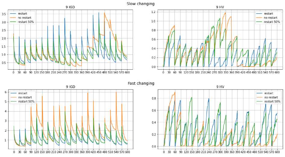
Рис. 6. Изменение значений метрик на примере задачи DF9 при медленных и быстрых изменениях

Fig. 6. Changing values of IGD and HV metrics in DF9 problem in the cases of slow and fast changes

With rapid changes in tasks DF1 and DF9, you can see that in the absence of a restart, the error value when changes occur is much higher compared to using a restart. Also in problem DF9 with slow changes it is seen that at the first iterations algorithm in the absence of a restart, a low error value is observed, however, at subsequent steps of the algorithm, the error increases. This suggests that within the same problem, it is necessary to use different approaches depending on the degree of changes that occur.

Conclusion

On a set of test problems of multi-criteria non-stationary optimization using the NSGA-2 and SPEA2 algorithms, three approaches to the formation of a population in emergence of changes in the problem were considered. It was shown that the efficiency of using a population of solutions obtained at a previous point in time depends on the rate of change in the problem.

With slow changes on most test problems, the best result is shown by the approach that involves the use of a population consisting only of solutions obtained at the previous point in time, since the type of problem does not change much. However, with rapid changes, it is not possible to single out any of the three possible approaches as preferable, since all three approaches have approximately the same ratio of test problems in which their use was the most effective. This implies the need to track the intensity of changes occurring in the task, and on the basis of this information to make a choice in favor of one or another approach to forming a population.