The environmental Phillips curve hypothesis for Russia: The relationship between the levels of environmental pollution and unemployment

The industrial revolution that emerged in the late 18th century brought with it many economic and social changes (Philbeck, Davis, 2018). With the industrial revolution, the production of goods and services increased rapidly, economic growth rates and welfare levels increased, developments in science and technology accelerated, population increases occurred, and cities became the centers of life (Dogaru, 2020). Although the industrial revolution had positive effects, it is also a fact that it had negative effects. Increases in the production of goods and services have not only brought about the rapid depletion of natural resources but also caused the accumulation of environmentally harmful waste because of production (Dimanov, 2024). Countries have long ignored the environmental damage caused by increased production to achieve high growth rates in a short time. However, over time, the damage caused by economic activities to the environment has reached great levels (Smolovic et al., 2023). The increase in environmental pollution threatens human health, causes a decrease in biological diversity, harms the quality of soil and water, and increases air pollution (Li et al., 2025). This has produced a necessity to pursue a new goal. Countries have begun to develop policies aiming to reduce environmental pollution (Winter, 2024). New concepts and policy approaches have emerged, such as sustainable growth, sustainable development, green economy, green growth, and circular economy. All these concepts are based on the relationship between the economy and the environment and aim to restructure production systems in a way that does not increase environmental pollution (Adamowicz, 2022).

Since the main reason for the increase in environmental pollution is humans, a wide literature has been formed on the effect of economic indicators on environmental pollution (Osuntuyi, Lean, 2023). Various theories aiming to explain the economy-environment relationship have emerged. There are hundreds of empirical studies examining the environmental Kuznets curve, the pollution haven hypothesis, and the pollution halo hypothesis, which are among these theories (Abbass et al., 2022).

The environmental Kuznets curve hypothesis is an improved version of the Kuznets curve introduced by Simon Kuznets (1955). In his study, Kuznets concluded that there is an inverted U-shaped relationship between per capita income and income inequality (Rayhan et al., 2020). Income inequality increases as per capita income increases. However, over time, per capita income reaches a turning point, and after this point, as per capita income increases, income inequality begins to decrease. In their study, (Grossman, Krueger, 1991) found an inverted U-shaped relationship between per capita income and environmental pollution. As income per capita increases, environmental pollution increases (Adhikari et al., 2024). After per capita income reaches a certain level, as per capita income continues to increase, environmental pollution decreases (Nica et al.,

2025). This hypothesis is called the environmental Kuznets curve because the relationship between income increases, and environmental pollution is similar to the relationship between income increase and income inequality (Wang et al., 2024).

According to the pollution haven hypothesis, some companies located in developed countries and operating in industries that create pollution direct their investments to developing countries (Murshed, 2025). The main reason for this is that developing countries generally lack strict environmental regulations and have low environmental standards (Bagchi, Sahu, 2025). Thus, foreign direct investment goes from developed countries to developing countries. While direct foreign investments are increasing in developing countries, environmental pollution is also increasing. Developing countries are becoming pollution havens for developed countries (Niu, Wang, 2024). According to this hypothesis, as foreign direct investment increases, environmental pollution increases and environmental quality decreases (Sreenu, 2025).

The pollution halo hypothesis, on the other hand, argues that an increase in foreign direct investments will reduce environmental pollution (Mishra et al., 2025). Foreign direct investments flowing from developed countries to developing countries bring with them new technologies (Achuo, Ojong, 2025). With the transfer of newer and more advanced technologies to developing countries, these countries have less polluting production processes. Environmental pollution is decreasing in developing countries with the adoption of nonpolluting production technologies. In other words, the pollution halo hypothesis states that there is an inverse relationship between foreign direct investments and environmental pollution (Ali, Wang, 2024).

A new one has been added in recent years to the hypotheses explained above, which examine the relationship between economic indicators and environmental pollution. Based on the Phillips curve (1958) theory, M. Kashem and M. Rahman (Kashem, Rahman, 2020) put forward a new hypothesis called the environmental Phillips curve. The Phillips curve is a theory that reveals the relationship between the inflation rate and the unemployment rate. According to the Phillips curve theory, there is a negative relationship between inflation and unemployment (Rayhan et al., 2020). The work (Kashem, Rahman, 2020) examining the relationship between environmental pollution and unemployment, found a negative relationship between these two variables. Due to the negative relationship between unemployment and environmental pollution, they named this hypothesis the environmental Phillips curve hypothesis (Shastri et al., 2023).

Environmental pollution and unemployment are two important problems that countries are struggling with. However, reducing environmental pollution and reducing unemployment are two objectives that cannot be achieved at the same time. For this reason, countries must choose which of these two tasks to solve. The environmental Phillips curve is extremely important as it gives a new perspective to the traditional Phillips curve and reveals the negative relationship between unemployment and environmental pollution (Shang, Xu, 2022). With the emergence of the environmental Phillips curve hypothesis in 2020, the number of studies testing the validity of this hypothesis has started to increase rapidly. However, since the environmental Phillips curve hypothesis is a relatively new hypothesis, it can be stated that empirical studies on this subject are still inadequate and more studies testing the hypothesis are needed. To compare the results and reach correct conclusions about the countries, studies should be conducted on different countries or country groups. To fill the gap in the literature, analyses that focus on countries or country groups that have not been examined before should be preferred. This study investigates the environmental Phillips curve hypothesis for Russia. Because of the literature review, no empirical study was found that tested the environmental Phillips curve hypothesis for Russia. It is thought that this study will contribute to the literature in this respect.

Russia is a country that has a great impact on the increase in CO2 emissions and greenhouse gases. The countries that emit the most greenhouse gases in the world are China, the United States, and India. After these countries, Russia comes. In terms of CO2 emissions, Russia causes CO2 emissions in the world to increase by approximately 7% (Magazzino et al., 2023). For this reason, analyzing indicators related to environmental pollution in Russia is important in terms of establishing environmental policies. Factors that increase environmental pollution must be reduced, and factors that contribute to the improvement of environmental quality must be supported. If the degree of impact of factors related to environmental pollution and the direction of the impact are determined correctly, more sound decisions can be made for the future policies. CO2 emissions were used as the dependent variable (an indicator of environmental pollution). The independent variable is the unemployment rate. Besides, different indicators that affect environmental pollution are also included in the model as independent variables: economic growth, urbanization, and total energy supply. The analysis covers the period after the dissolution of the Soviet Union: 1992–2022. The method Fourier Augmented ARDL approach was used.

Literature review

Although there are many studies testing the environmental Kuznets curve hypothesis in the literature, this issue continues to attract attention today (Biyase et al., 2024; Amankwa et al., 2024; Horobet et al., 2024; Rabbi, Abdullah, 2024; Khalid et al., 2025; Kolasa-Wiecek et al., 2024; Menegaki et al., 2025; Naqvi et al., 2025; Odei et al., 2025; Porto et al., 2025). Similarly, the number of studies on the pollution haven hypothesis and the pollution halo hypothesis continues to increase (Gogoi, Hussain, 2024; Padhan, Bhat, 2024; Forson, 2024; Kumar et al., 2024; Balla, Lokonon, 2024; Holtbrugge, Raghavan, 2025; Al Numan et al., 2025; Ekesiobi et al., 2025; Dar et al., 2025; Soti et al., 2024).

As noted earlier, the environmental Phillips curve hypothesis was proposed in the article (Kashem, Rahman, 2020). When the studies in the literature are examined, it is seen that different indicators such as CO2 emission, ecological footprint, and load capacity factor are used as indicators of environmental pollution. Additionally, the models include different independent variables: economic growth, foreign direct investments, renewable energy consumption, population growth, urbanization, and globalization; their impact is compared with the impact of unemployment. Below, information about studies on the environmental Phillips curve hypothesis is presented.

(Bhowmik et al., 2022) examined the validity of the environmental Phillips curve hypothesis for the United States. They used CO2 emissions as a pollution indicator. By applying ARDL analysis, the relationship between environmental pollution and unemployment was researched for both the short and long term. In the United States, the environmental Phillips curve hypothesis is valid eventually but not in the short run. For this reason, it appears that the relationship between environmental pollution and unemployment differs in the short and long term (Bhowmik et al., 2022).

(Tanveer et al, 2022) investigated the relationship between environmental pollution and unemployment in Pakistan. In the study, three different environmental indicators were used: CO2, CH4 and the ecological footprint. In addition to unemployment, energy consumption, foreign direct investments, economic growth, and globalization were added to the model as independent variables. According to the results of the analysis covering the period of 1975–2014, the environmental Phillips curve hypothesis is valid for Pakistan. In the long run, direct foreign investments affect environmental sustainability positively, while globalization negatively affects it.

(Tariq et al., 2022) tested the validity of the environmental Phillips curve hypothesis for southern Asian countries. The dataset includes the period 1991–2019. The ecological footprint was used to represent environmental pollution, and ARDL analysis was performed as the method. Population growth, renewable energy use, non-renewable energy use and GDP are other independent variables in the model. The results of the analysis reveal that the environmental Phillips curve hypothesis is valid for south Asian countries. There is a negative correlation between unemployment and environmental pollution (Tariq et al., 2022).

(Haciimamoglu, 2023) tested the validity of the environmental Phillips curve hypothesis by examining the relationship between environmental pollution and unemployment in the Next-11 countries. The ecological footprint was used as an environmental pollution indicator. In the Next-11 countries, there is a negative relationship between environmental pollution and unemployment. This result indicates that the environmental Phillips curve hypothesis is valid.

(Durani et al., 2023) tested the validity of the environmental Phillips curve hypothesis in their analysis for the BRICS-T countries. The dataset used in the study covers the 1990–2020 period. CO2 emissions were used as environmental pollution indicators. In addition to employment, indicators regarding economic policy uncertainty, renewable energy use, financial development, technological progress and natural resource rents are included in the model. Employment and financial development in BRICS-T countries increase CO2 emissions while the use of renewable energy and economic policy uncertainty decrease them.

(Addison et al., 2024) studied the relationship between environmental quality and unemployment in Ghana. ARDL analysis was applied using a data set covering the 1990–2019 period. According to the analysis results, the effects of the total unemployment rate, female unemployment, and male unemployment on environmental quality are different. Therefore, the study concluded that the environmental Phillips curve hypothesis is not valid for Ghana (Addison et al., 2024).

(Yavuz et al., 2024) tested the environmental Phillips curve hypothesis for Turkiye. The load capacity factor was used in the study instead of the carbon emission or ecological footprint. Thus, it aimed to focus on environmental quality rather than environmental pollution. A dataset covering the period 1982–2022 was used. A-ARDL was used as a method. The analysis results show that the environmental Phillips curve hypothesis is valid for Turkiye (Yavuz et al., 2024).

(Kinnunen et al., 2024) explored the validity of the environmental Phillips curve hypothesis for Finland. ARDL analysis was applied using data covering the 1990–2022 period. In addition to the unemployment rate, renewable energy consumption, urbanization, and GDP per capita are included in the model. The environmental Phillips curve hypothesis has been found not to be valid in Finland (Kinnunen et al., 2024).

(Da§tan, Eygu, 2024) tested the validity of the environmental Kuznets curve and the environmental Phillips curve for Turkiye. The A-ARDL method was applied using data covering the period 1980–2018 from Turkiye. The ecological footprint has been included in the model as an indicator of environmental pollution. According to the analysis results, both hypotheses are valid for Turkiye. In addition, while urbanization, which is one of the other independent variables added to the model, helps to increase the environmental quality, natural resource rents deteriorate the environmental quality by increasing the ecological footprint (Da§tan, Eygu, 2024).

(Golkhandan, 2024) explored the relationship between environmental pollution and unemployment for countries in the MENA region. There is an analysis covering data from 11 countries in the MENA region for the period 2000–2022. The load capacity factor was preferred as an environmental pollution indicator. For this reason, the validity of the load capacity curve hypothesis was also examined in the study. It was concluded that the environmental Phillips curve hypothesis cannot be rejected in the examined countries. Additionally, the load capacity curve hypothesis was found to be valid. The panel causality analysis shows that there is a two-way causality between unemployment and the load capacity factor (Golkhandan, 2024).

(Azimi, Rahman, 2024) investigated whether the environmental Phillips curve hypothesis is valid in the G7 countries. CO2 emissions were used as environmental pollution indicators. The data set covered the period 1990–2022. CS-ARDL, wavelet coherence, and wavelet causality analyzes were applied. The obtained findings show that the hypothesis is valid in the G7 countries.

(Ayad, Djedaiet, 2024) present another study that examines the environmental Phillips curve hypothesis for G7 countries. Unlike (Azimi, Rahman, 2024), the study used the load capacity factor as an environmental indicator. Therefore, analysis was conducted to test both the environmental Phillips curve hypothesis and the load capacity curve. According to the results of the PMG-ARDL and CS-ARDL analysis, both hypotheses are valid in the G7 countries (Ayad, Djedaiet, 2024).

(Sahin et al., 2025) used data from the 10 developing countries with the highest carbon emissions to test the environmental Phillips curve hypothesis. The dataset covered 1990– 2019. They applied ARDL analysis and found an inverse relationship between unemployment and environmental degradation. Thus, the environmental Phillips curve hypothesis is valid in the examined countries (Sahin et al., 2025).

(Koyuncu Qakmak et al., 2025) tested the environmental Phillips curve hypothesis for developed and developing countries for the period 1990–2020. According to the results of the analysis, the environmental Phillips curve hypothesis is not valid in both the short and long term in high-income countries. However, the environmental Phillips curve hypothesis is valid in upper middle and lower middle-income countries (Koyuncu Qakmak et al., 2025).

The research results described above are summarized in Table 1 . According to the data presented, the environmental Phillips curve hypothesis is generally confirmed, while the number of countries where it is refuted is decreasing.

Data and methods

In this study, Fourier Augmented ARDL Bounds Test approach was used to analyze the long-run relationship between unemployment and environmental pollution in Russia. The analysis covers the 1992–2022 period. Carbon emissions were used to represent environmental pollution and as the dependent variable. The independent variable is the unemployment rate. Moreover, economic growth, total energy supply, and urbanization was added to the model as control variables. Logarithmic conversions of the variables were used in the analysis. The model of the study, which was created based on the studies carried out in (Kashem, Rahman, 2020; Kinnunen et al., 2024; Da§tan, Eygu, 2024), is shown with equation (1).

CO_2t = /? o + P i GDP_t + ?₂ES_t + p₃URB_t + +&UNP_t + s t , ⁽¹⁾

where: CO ₂ – carbon emissions (metric tons per capita); GDP – economic growth (GDP per capita, constant 2015 USD); ES – total energy supply (million tons of oil equivalent); URB – urbanization (% of total population); UNP – unemployment (percentage of the labor force); £ _t — error term. Table 2 contains descriptions of the variables and data sources.

Table 1. Studies testing the environmental Phillips curve hypothesis

Author/Authors (Year)	Country/Countries	Method	Findings
(Kashem, Rahman, 2020)	30 industrialized countries	OLS	The environmental Phillips curve hypothesis is valid for industrialized countries.
(Bhowmik et al., 2022)	United States	ARDL	The environmental Phillips curve hypothesis is eventually valid but not in the short run.
(Tanveer et al., 2022)	Pakistan	ARDL	The environmental Phillips curve hypothesis is valid in Pakistan.
(Tariq et al., 2022)	Southern Asian countries	Panel ARDL	The environmental Phillips curve hypothesis is valid for South Asian countries.
(Hac i imamo g lu, 2023)	Next-11 countries	AMG, DCCE	The environmental Phillips curve hypothesis is valid.
(Durani et al., 2023)	BRICS-T countries	FMOLS, DOLS	The environmental Phillips curve hypothesis is valid for the BRICS-T countries.
(Addison et al., 2024)	Ghana	ARDL	The environmental Phillips curve hypothesis is not valid in Ghana.
(Yavuz et al., 2024)	T u rkiye	A-ARDL	The environmental Phillips curve hypothesis is valid for T u rkiye.
(Kinnunen et al., 2024)	Finland	ARDL	The environmental Phillips curve hypothesis is not valid in Finland.
(Da ? tan, Eyg u , 2024)	T u rkiye	A-ARDL	The environmental Phillips curve hypothesis is valid in T u rkiye.
(Golkhandan, 2024)	11 countries in the Middle East and North Africa	PMG-ARDL, PMG-NARDL	The environmental Phillips curve hypothesis is valid in the countries examined.
(Azimi, Rahman, 2024)	G7 countries	CS-ARDL, Wavelet Coherence, and Wavelet Causality	The environmental Phillips curve hypothesis is valid in the G7 countries.
(Ayad, Djedaiet, 2024)	G7 countries	PMG-ARDL, CS-ARDL	The environmental Phillips curve hypothesis is valid in the G7 countries.
(Sahin et al., 2025)	10 developing countries	Panel ARDL	The environmental Phillips curve hypothesis is valid in the countries examined.
(Koyuncu Q akmak et al., 2025)	Developed and developing countries	Dynamic Panel ARDL	In high-income countries, the environmental Phillips curve hypothesis is not valid in both the short and long term. However, the environmental Phillips curve hypothesis is valid in upper middle and lower middle-income countries.
Source: own elaboration.

Table 2. Variable specification

Acronym	Variable	Measurement Unit	Source
CO 2	Carbon emission	Metric tons per capita	World Bank
GDP	Economic growth	GDP per capita, constant 2015 USD	World Bank
ES	Total energy supply	Million tons of oil equivalent	OECD
UR B	Urbanization	Urban population (% of total population)	World Bank
UNP	Unemployment	Percentage of the labor force	World Bank
Source: own elaboration.

In time series analysis, it is important to examine the stationarity characteristics of the series. Classical unit root tests (Augmented Dickey – Fuller, ADF) can give misleading results in the presence of structural breaks in the series. Especially if there are structural breaks that are not sudden, have a smooth transition, or change over time, the explanatory power of these tests’ decreases. To solve this problem, the authors (Christopoulos, Leon-Ledesma, 2010) developed the Fourier ADF (Augmented Dickey – Fuller) unit root test. This test is an extension of the traditional ADF test, aiming to show possible structural breaks and periodic components in the time series more clearly. This test models the deterministic trend component flexibly using Fourier series terms. It can also add structural changes to the model without requiring prior knowledge of the number, location, and shape of the breaks (Enders, Lee, 2012). Fourier series have a high ability to reveal potentially complex trends and seasonality. For this reason, it is a more flexible approach than the traditional linear or polynomial trends (Gallant, Souza, 1991). The Fourier ADF test is based on the regression model below:

r       s2rtkt\         s2nkt\]

^t = « о + « i ^t + / [Y i sm ^7- J + У 2 cos \^-^JJ +

^=1            ''                        , (2)

series; t – time trend; k – frequency; T – number of observations;

(2nkt\        ^2nkct\ sin (—^) ve cos (—^) — Fourier series terms; ρ –autoregressive coefficient;

p – number of augmented terms (lagged diffe- rences); q — error term. The main purpose of the test is to test the null hypothesis ρ = 0. If the null hypothesis is rejected, it is concluded that the series does not contain unit roots and therefore is stationary. Fourier terms were added to the model to capture potential structural breaks and nonlinear movements in the series. The number of frequencies

( k ) is determined empirically and is usually chosen based on information criteria or the significance of the test statistics (Christopoulos, Leon-Ledesma, 2010).

The Fourier Augmented ARDL (FAARDL) approach is a method developed to analyze long term co-integration relationships between variables and aims to overcome some limitations of the traditional ARDL model. The standard ARDL bounds test (Pesaran et al., 2001) can lose reliability, especially in the presence of non-stationary structural changes, making it difficult for the model to accurately detect long term relationships. Furthermore, the traditional ARDL model has significant disadvantages, such as the requirement that the dependent variable be I (1) and the disregard for degenerative structures and structural breaks that may arise when a large number of independent variables are included in the model. In this context, the extended ARDL approach developed in (McNown et al., 2018) and (Sam et al., 2019) allows for the detection of degenerative situations by adding the FB test for the lagged levels of the independent variables. The Fourier ARDL model, on the other hand, integrates Fourier terms into this structure, making it possible to model structural breaks with particularly smooth transitions, thus significantly increasing the model’s flexibility (Enders, Lee, 2012; Yilanci et al., 2020; Syed et al., 2023; Apergis et al., 2023).

Thanks to this advanced structure, FAARDL not only considers structural breaks but also offers the flexibility to work with different levels of stationarity. This feature provides a significant advantage, particularly in the analysis of time series in complex economic systems. It also offers effective solutions to problems encountered in traditional ARDL models, such as small sample size and low test power. The bootstrap simulations used in the FARDL model allow for a more reliable assessment of the significance of test statistics and eliminate the uncertainties encountered in tests based on asymptotic critical values (Wu et al., 2022; Lin, Wu, 2022). The model can produce more robust results, both theoretically and empirically (Kumar, Patel, 2024).

As a result, the Fourier-augmented ARDL approach stands out due to its advantages, such as its ability to flexibly model structural breaks, to work with series with different degrees of integration, and to offer high test power even in small samples (Nazir, 2024; Goh et al., 2017). In this way, the potential for the existence of structural breaks in time series analyses to negatively affect the reliability of traditional cointegration tests and standard ARDL results can be eliminated, and the relationships between variables can be analyzed on a more solid basis (Yilanci et al., 2020; Bozatli, Ak^a, 2024). The FAARDL method is distinguished from similar models by its ability to flexibly represent structural breaks within the model without requiring any prior knowledge about the timing of these breaks. This flexibility allows researchers to conduct more accurate and reliable analyses, especially in economic systems experiencing sudden regime changes, thus contributing to the development of more accurate predictions for policy and decision makers (Georgescu, Kinnunen, 2024).

The model created in (Pesaran et al., 2001) based on equation (1) is as follows:

^C02_t = « 0 + <₁ft4C02_t - _; + Si^GDP i- + +s ^ ₁8_iaEs_t-i + s^V i auRB t—i + ^₌₁e_iAUNP_t-i +

, (3) +A₁4C02_t-1 + A₂4GDP_t-1 + A₃4ES_t-1 + A₄AURB_t-1 +

+As^UNPt—i + £t where: a0 — constant coefficient; J — first differences; βi, γi, δi, φi, θi – short-term coefficients; λi (i = 1, 2, 3, 4, 5) – long-term coefficients; k, l, m, n, p – lag length according to the AIC information criterion (Akaike, 1979); £t — error term.

M. Pesaran and co-authors (Pesaran et al., 2001) presented two co-integration tests.

T-test for the dependent variable:

H o : ^ i = 0                                    (4)

FA-test for all variables:

H_o : 2 1 = 2 ₂ = 2 3 = 2 ₄ = 2 5 = 0.                (5)

The work (Sam et al., 2019) proposed a FB test for independent variables at the lagged level in the Augmented ARDL method to support t and F tests.

FB-test for independent variables:

H₀ : 2 ₂ = 2 3 = 2 ₄ = 2 5 = 0.                    (6)

(Sam et al., 2019) proposed these three ways to define cointegration, non-cointegration, and degeneration. If these three tests (t-test, FA-test, FB-test) reject the H0 hypothesis, cointegration occurs. In the Augmented ARDL model, the deterministic component in equation (7) was added to the model in order to take breaks into account with smooth transitions. Because of this arrangement, equation (8) was finally obtained (Yilanci et al, 2020).

/2nkt\ ,    _ fknkt\

d(t)= Yism[—) + / 2 cos(—J .    (7)

ACO2_t = a₀ + y₁sin

(2?)

f 2nkt

+ V i cos (—) + SK 1WCO2 —

+S^l_l= i_{Y l}&GDP t— _l + S^i S^ES — + ^i^URB t—, + +S^p_i=10_lAUNP_t-l + A 1 ACO2_t-1 + A₂AGDP_t-1 + L 3 AES_t-1

. (8)

+

+A₄AURB_t-1 + A 5 AUNP_t-1 + e_t

In equation (8): π = 3.14 – constant; k – number of selected specific frequencies, t – trend; T – number of observations.

In the study, first the descriptive statistics of the variables were examined ( Tab. 3 ). GDP has the highest mean (8.901), while UNP has the lowest mean (1.931). UNP has the highest standard deviation (0.317) while URB has the lowest standard deviation (0.007). This shows that the urbanization rate is fairly stable throughout the sample. Skewness values indicate the direction and degree of deviation

Table 3. Descriptive statistics

Variables	CO2 (tons per capita)	GDP (GDP per capita, constant 2015 USD)	ES (million tons of oil equivalent)	URB (urban population,% of total population)	UNP (percentage of the labor force)
Mean	2.411	8.901	6.529	4.301	1.931
Median	2.422	9.034	6.534	4.298	1.883
Maximum	2.581	9.231	6.712	4.319	2.585
Minimum	2.295	8.415	6.377	4.295	1.352
Std. dev.	0.067	0.284	0.088	0.007	0.317
Skewness	0.32	-0.446	0.302	1.214	0.422
Kurtosis	3.063	1.594	2.297	3.32	2.4
Jarque–Bera	0.534	3.579	1.111	7.747	1.383
Probability	0.766	0.167	0.574	0.021	0.501
Source: own calculation.

from the symmetry of the distributions of the variables. For example, the positive skewness of URB (1.214) indicates that the distribution is skewed to the right, while the negative skewness of GDP (-0.446) indicates a skewness to the left. The kurtosis value of GDP is 1.594; therefore, it is platykurtic. The Jarque – Bera test and probability values test whether the variables exhibit a normal distribution. The low probability value of the URB variable (0.021) indicates that this variable deviates significantly from the normal distribution. Since the probability values of the other variables are above the 5% significance level, the normal distribution hypothesis of these variables cannot be rejected.

The correlation matrix (Tab. 4) shows the relationships between the variables. According to the matrix, there are significant linear relationships between the macroeconomic variables examined. In particular, the high positive correlation between ES and CO2 emissions (r = 0.906) supports the energy-environment relationship hypothesis in the literature. The positive correlations between GDP and CO2 and GDP and ES (r = 0.563 and r = 0.725, respectively) indicate that economic growth may have environmental impacts. Strong negative correlations between UNP and all other variables create an expectation that unemployment may decrease as economic performance improves and energy consumption increases. These correlation findings highlight the importance of examining potential co-integration relationships and causality relationships between variables in more depth through econometric analyses.

Table 4. Correlation matrix

	CO 2	GDP	ES	URB	UNP
CO2	1.000
GDP	0.563	1.000
ES	0.906	0.725	1.000
URB	0.458	0.751	0.749	1.000
UNP	-0.829	-0.852	-0.915	-0.748	1.000
Source: own calculation.

Results

In order to empirically determine the stationarity properties of the series in the study, modern approaches that consider structural breaks were applied in addition to traditional unit root tests. The Augmented Dickey – Fuller (ADF) unit root test (Dickey, Fuller, 1981) was used to test the stationarity of the series. In addition, in order to obtain more reliable results by considering the effects of possible structural breaks in the time series, the Fourier ADF unit root test proposed in (Christopoulos, Leon-Ledesma, 2010) was also applied. The stationarity test results are given in Table 5.

The Fourier ADF test results indicate the presence of non-linear trends in the all-time series examined, as the F test statistics are above the 5% critical value (Becker et al., 2006). However, the FADF statistics of the same test reveal that no variable is stationary at the level when the 5% critical value is considered. This shows that the variables contain a unit root in their original form even when the Fourier terms are considered.

The findings of the traditional ADF test also support this result. None of the variables are stationary at the 5% significance level, but when the first differences of all the variables are taken, they become stationary at the 5% significance level. Therefore, both the Fourier ADF and traditional ADF test results show that the examined variables are stationary in their first differences, that is, I (1). These results show that the variables are suitable for the Fourier augmented ARDL bounds test analysis and that potential long-run relationships (cointegration) between the variables can be examined.

Since the series were determined to be stationary in the first difference, the Fourier Augmented ARDL bounds testing approach was used in the analysis of the long-term relationships between the variables. This method can be used in series with different degrees of stationarity (I (0) or I (1)). Moreover, thanks to the soft structural breaks included in the model provide more reliable cointegration results by considering the effects of possible economic and political changes over time (Aliyev et al., 2024).

Table 5. Fourier ADF and ADF unit root test results

Variables	Fourier ADF			ADF
	Level			Level		First difference
	Frequency (k)	FADF test statistics	F test statistics	Test statistics		Test statistics
CO 2	1	-3.466	11.636	-2.499 (0.125)		-4.181(0.002)***
GDP	1	-0.944	63.820	-0.974 (0.748)		-3.332 (0.022)**
ES	1	-2.541	24.070	-1.345 (0.595)		-4.498 (0.001)***
URB	1	-0.551	20.484	-2.354 (0.999)		-3.286 (0.025)**
UNP	1	-2.366	26.045	-0.729 (0.824)		-3.811 (0.007)***
Critical values	FADF test statistics				F test statistics
k: 1	%1 [4.43], %5 [3.85], %10 [3.52]				%1 [6.730], %5 [4.929], %10 [4.133]

Note: *** p<0.01, ** p<0.05, * p<0.1.

Source: own calculation.

Table 6 shows the Fourier-augmented ARDL bounds test results. The optimal lag lengths used in the model are specified separately for the dependent and independent variables. In this study, CO₂ emissions are the dependent variable and all other variables (GDP, ES, URB, UNP) are independent variables. The Fourier frequency (k) is determined as 1.3. This value is assumed to represent the frequency of the potential structural breaks and nonlinear movements in the series.

The table includes FA statistics (Narayan, 2005), t-statistics (Pesaran et al., 2001) and FB statistics (Sam et al., 2019). The FA statistic (45.543) is considerably larger than the upper bound critical values (6.670, 4.774 and 3.994, respectively) at the 1%, 5% and 10% significance levels presented for both I (0) and I (1). This result shows that the null hypothesis (that there is no long-run relationship between the variables) is strongly rejected at all significance levels. Therefore, there is a long run co-integration relationship between CO2 emissions and GDP, ES, URB and UNP.

The t-statistic (-11.275) is greater than the lower and upper critical values (-3.43 and -4.60; -2.86 and -3.99; -2.57 and -3.66, respectively) at the 1%, 5% and 10% significance levels for both I (0) and I (1). This means that the coefficient of the dependent variable CO2 is not zero and is significantly included in the long-term model.

The FB statistic (49.809) is the result of the additional F-test applied to the lagged levels of the independent variables to test for degenerative states. This statistic is also significantly greater than the upper critical values (6.83, 4.70 and 3.84, respectively) at all significance levels. This result shows that there is no degenerative situation in the model and the co-integration results obtained are reliable.

As a result, the Fourier Augmented ARDL bounds test findings prove the existence of a statistically significant and robust long run cointegration relationship between CO2 emissions and economic growth (GDP), energy supply (ES), urbanization (URB), and unemployment (UNP). The fact that the model includes Fourier terms means that possible structural breaks are also considered when testing the existence of this longterm relationship. High FA and FB statistics indicate that the model strongly supports co-integration and is free from degenerative problems.

Table 7 shows the long-term coefficients of the Fourier Augmented ARDL bounds test. According to the table, the long-term coefficient of economic growth (GDP) is -0.241 and this coefficient is statistically significant at the 1% significance level (p=0.000). In Russia, a 1% increase in GDP eventually leads to a decrease in CO₂ emissions of approximately 0.241%, all other variables being

Table 6. Fourier Augmented ARDL cointegration test results

Lag Length	Frequency (k)		FA		t-Statistic		F B
1, 0, 0, 0, 0	1.3		45.543***		-11.275***		49.809***
Table critical values	Lower bound I (0)				Upper bound I (1)
	%1	%5		%10	%1	%5		%10
F A	4.768	3.354		2.752	6.670	4.774		3.994
t-Statistic	-3.43	-2.86		-2.57	-4.60	-3.99		-3.66
F B	4.15	2.80		2.22	6.83	4.70		3.84
Note: *** p < 0.01, ** p < 0.05, * p < 0.1. Source: own calculation.

Table 7. Fourier Augmented ARDL long-term coefficient results

Model: CO2 = f (GDP, ES, URB, UNP)
Variables	Coefficient	Std. error	t-statistic	Prob.
GDP	-0.241	0.061	-3.970	0.000***
ES	0.663	0.104	6.402	0.000***
URB	2.654	2.008	1.470	0.156
UNP	-0.108	0.031	-3.547	0.001***
CointEq (-1)	-0.945	0.056	-16.719	0.000***
Note: *** p<0.01, ** p<0.05, * p<0.1. Source: own calculation.

constant. While a positive relationship is generally expected between economic growth and CO2 emissions, the negative coefficient obtained here is striking. This situation can be related to factors such as the shift of industrial production to less polluting sectors with economic development, increases in energy efficiency, technological advances, or the effectiveness of environmental regulations. The results highlight the complexity and countryspecific dynamics of the relationship between growth and environmental quality.

The long-term coefficient of energy supply (ES) is 0.663, which is statistically significant at the 1% significance level (p=0.000). In the long run, a 1% increase in the energy supply increases approximately 0.663% in CO2 emissions, with other variables remaining constant. Considering that energy production and consumption are one of the main determinants of CO2 emissions, this positive and significant relationship is an expected result. The fact that Russia is an energy-intensive economy and production relies heavily on fossil fuels supports the finding that increases in energy supply directly and significantly increase CO2 emissions. This result reveals the importance of measures targeting the energy sector in CO2 emission reduction policies.

The long-term coefficient of the urbanization rate (URB) is 2.654, but this coefficient is not statistically significant (p=0.156). Although the coefficient is positive, there is not enough evidence to prove that urbanization has a statistically significant effect on CO2 emissions eventually within the framework of the model used in the study. The environmental impacts of urbanization are often complex. On the one hand, urbanization can increase energy consumption and emissions from transportation, and on the other hand, it can enable the development of more efficient infrastructures and public transportation systems.

The long-term coefficient of unemployment (UNP) is -0.108 and this coefficient is statistically significant at the 1% significance level (p=0.001). In the long run, a 1% increase in the unemployment rate decreases CO2 emissions of approximately 0.108%, other variables being constant. This finding reflects the expected negative relationship between economic activities and environmental pollution. The analysis results support the validity of the environmental Philips curve hypothesis in Russia. The environmental Phillips curve hypothesis claims that there is a negative relationship between unemployment and environmental pollution. An economic recession or slowdown can have environmental impacts. The finding that the environmental Philips curve is valid for Russia supports the studies (Kashem, Rahman, 2020; Bhowmik et al., 2022; Tanveer et al., 2022; Tariq et al., 2022; Haciimamoglu, 2023; Durani et al., 2023; Yavuz et al., 2024; Da§tan, Eygu, 2024; Golkhandan, 2024; Azimi, Rahman, 2024; Ayad, Djedaiet, 2024; Sahin et al., 2025; Koyuncu Qakmak et al., 2025).

The error correction term of the model is -0.945 and is significant at the 1% level. According to this finding, there is a strong long-term co-integration relationship between the variables in the model. Approximately 94.5% of the deviations occurring in the short term are corrected in the next period and the system rapidly approaches the long-term equilibrium. Russia should align its economic growth with environmental sustainability by investing in energy efficiency and clean energy technologies.

The diagnostic test results in Table 8 reveal the reliability and validity of the Fourier ARDL model applied in the study. The Jarque – Bera (JB) test shows that the residual terms are normally distributed, the Breusch – Godfrey – Lagrange Multiplier (BG-LM) test shows that there is no autocorrelation in the model, and the Breusch –

Pagan – Godfrey (BPG) test shows that there is no heteroscedasticity. The Ramsey RESET (RR) test indicates that the functional form of the model is established correctly.

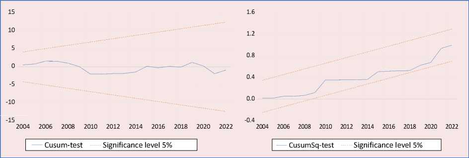
The stable results of the CUSUM and CUSUM of Squares (CusumSq) tests in the Figure indicate that the model coefficients remained stable over time and there was no structural break. These findings prove that the estimated model is statistically robust and reliable.

Conclusion and recommendations

The environmental Phillips curve hypothesis reveals an inverse relationship between unemployment and environmental pollution. In this study, the environmental Phillips curve hypothesis was examined for Russia. Fourier Augmented ARDL analysis was applied using data covering the period 1992–2022. CO2 emissions, which are

Table 8. Diagnostic tests

Tests	Test statistics	Prob.
JB	0.396	0.820
BG-LM	0.286	0.753
BPG	0.492	0.830
RR	0.494	0.626
Cusum: stable		CusumSq: stable
Source: own calculation.

Cusum and CusumSq graphs

used as an environmental pollution indicator in the model, are the dependent variable. The independent variables are the unemployment rate, urbanization rate, total energy supply and economic growth. According to the analysis results, the environmental Phillips curve hypothesis is valid in Russia. There is an inverse relationship between the unemployment rate and environmental pollution. An increase in economic growth decreases environmental pollution. However, urbanization and the increase in the total energy supply increase environmental pollution.

Reducing unemployment and lowering environmental pollution are priority goals for many countries. However, according to the environmental Phillips curve hypothesis, it is impossible to achieve both these goals simultaneously. The most optimal step in this direction is improving employment policies while considering environmental objectives. Possible measures include increasing investments in renewable energy sources, especially in regions with high unemployment, and expanding production in sectors that do not lead to increased pollution levels. Changing the employment structure through the reallocation of labor from heavily polluting economic sectors to more environmentally friendly ones is also an option. This process requires time and should be implemented gradually. Its successful completion necessitates long-term planning and a clear outline of the process stages.

In recent years, new professions called green jobs have emerged in line with the goals of sustainable development, a green economy and growth. Green jobs both protect the workforce by embodying features befitting human dignity and include production activities that attach importance to the protection of the environment. Establishing employment policies focused on green jobs in Russia could be an important step in combating environmental pollution. Since green jobs require characteristics such as the use of technology, environmental awareness, technical knowledge, creativity, teamwork, and easy adaptation to new conditions, the education system can be rearranged to meet these requirements. Manufacturers who contribute to increasing green employment can be supported with various incentives. Advantages such as tax reductions and tax exemptions can be provided to companies that use production techniques that do not pollute the environment. Financial support can be provided to investors who want to invest in green technologies and green production systems. Because transforming production systems and integrating non-polluting technologies into the production process requires high costs. In order to cover this cost, producers can be offered long-term credit opportunities under suitable conditions. Since it is difficult for the necessary investments to be met by the private sector alone, practices that increase cooperation between the public and private sector can be implemented. The number of companies that use energy and natural resources more efficiently and increase their use of renewable energy should be increased. In this way, both environmental quality and new employment opportunities can be created.

Furthermore, within the framework of sustainable development policy, the share of renewable energy sources in the overall energy supply must be increased.

Although the level of urbanization positively correlates with the level of environmental pollution, this dependence is statistically insignificant. Nevertheless, the reorganization of urban policy and the establishment of a priority for creating “green cities” are extremely important directions for sustainable development. Such cities are more livable. In them, renewable energy sources power the transportation system, accumulated waste is converted into energy, water consumption is reduced, rainwater is collected and used efficiently, and the number of electric vehicles is growing. The spread of green cities can reduce the negative impact of urbanization processes on the environment. At the same time, implementing green city projects can create many new jobs and, consequently, contribute to the fight against unemployment.

Thus, the inverse relationship between the unemployment rate and the level of environmental pollution in Russia, which confirms the environmental Phillips curve hypothesis, can be used in the country’s interests through the adoption of appropriate measures. In other words, shaping employment policy in accordance with sustainable development principles can help combat environmental pollution without increasing the unemployment rate. It is necessary to conduct similar studies across Russia’s regions as well. Further research on the environmental Phillips curve hypothesis will contribute to a deeper investigation of this issue and fill gaps in the literature.