The Estimation and Experiment of Axial Force in Deep Well Pump Basing on Numerical Simulation

Published Online December 2010 in MECS

Thrust bearing, balance hole or balance drum, impeller symmetrical arrangement, associated vane s, balance disc and other methods were used in the design of a deep well pump to balance the axial force. The axial force prediction generally consists of experimental measurement and using of empirical formulas. However, the test costs lots of time and financial resources, and it’s low accuracy by using empirical formulas.

A certain type of deep well pump was simulated using fluent to obtain the pressure distribution of the entire flow field, and then value of the pump axial force was calculated. A device was designed to measure the axial force of well submersible pumps, which has a simple structure and accurate measurement. Compared with the two states under the axial force predicted and experimental values respectively, the maximum error of the whole condition is 6.2%. It indicates that it’s feasible to calculate the axial force of submersible pump by using numerical simulation.

• II.    Hydraulic model design and

Pre-processing of numerical simulation

A. Impeller design

The Pump basic design parameters: flow rate Q = 20 m³/h, Head H = 20 m, speed n = 2850 r/min, specific speed n s = 82.

The impeller was designed by a new hydraulic design method—head maximum approach. The axial plane of the impeller is shown in Fig.1. The diameter of the front shroud is a little smaller than that of the pump casing inner diameter and the impeller outlet is inclined. The main structural parameters are listed in Table 1.

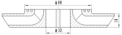
Figure 1. The axial projection drawing of impeller

TABLE I.

THE MAIN STRUCTURAL PARAMETERS OF IMPELLER

Impeller parameters	Specific value
Blade number Z	7
Blade inlet angle в 1 ( ° )	30
Blade outlet angle   в 2 ( ° )	35
Wrapping angle Ф ( ° )	115
Impeller diameter front cover D2max ( mm )	148
Impeller diameter back cover D2min ( mm )	132
Impeller inlet diameter D 1 ( mm )	62
Impeller outlet diameter b2 ( mm )	12
Impeller hub diameter dh ( mm )	38
Hydraulic radius front cover R 1 ( mm )	6
Hydraulic radius of the rear cover R 2 ( mm )	18
Shaft diameter d (mm )	28

National“863”project (2007AA05Z207), National science and technology supporting project (2008BAF34B15)

B. Hydraulic Design of guide vanes

In order to shorten the axial length of deep well pump, the radial guide vane is used. The main parameters are as follows: blade number Z=6 , inlet diameterD5 = 145 mm, outlet diameter D6 = 145 mm, inlet angle a 5 = 18 , outlet angle a6 = 58 , the axial projection drawing is shown in

Fig. 2.

E. Boundary conditions [1-4]

• Inlet boundary condition

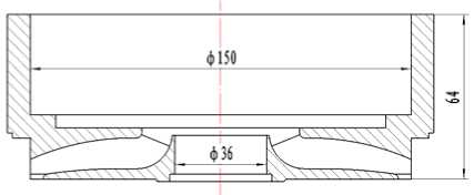
Figure 2. Axial projection drawing of guide vane

Inlet axial velocity is determined by the law of conservation of mass and assumption of rotational flow. Considering the relative motion of the impeller and flow, the relative velocity distribution of inlet section in the impeller is given. Supposing the pressure on the inlet section is uniform, the inlet of the turbulent kinetic energy k_in and turbulent kinetic energy dissipation rate are

calculated by the following formula [5]

' k in = 0.005 v 2

<          c ^3/4 k ^3/2

_   ----in-- e in

I Ky in

（ 1 ）

C. Solid Modeling

The hydro-equipment of 200QJ20 Type deep well pump is composed of the inlet section, impeller, guide vane and outlet section. The impeller and guide vane model are shown in Fig.3. Since grid generation can be directly affected by the quality of the 3-D model, the small planes, small acute angles and discontinuous surfaces should be avoided in modeling. In this simulation, the whole flow channel including the impeller, the guide vane and the cavity around the impeller cover was not simplified. And both the inlet and outlet section are enough extended, so the border of impeller blades inlet and outlet can not be affected by the inlet and outlet flow.

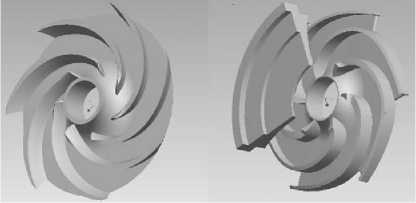
Figure 3. Solid model of impeller and guide vanes

Where: v _in is the inlet axial velocity; y _in is the distance between calculating point of near wall and wall surface.

• •    Outlet boundary condition

The flow rate and pressure in the outlet of guide vane of deep well pumps are unknown, so the flow outlet boundary condition is set to (outflow) form.

• •    Solid-wall condition

Considering the non-slip condition of solid-wall, the relative velocity w = 0, pressure is taken as the second boundary condition, that 8 p 1 8 n = 0. The turbulence wall boundary condition adopts wall function. Near the solid wall area, a large velocity gradient is forced by the wall. The full development k - e turbulence model in this region needs to be amended. Assuming the distance between near wall point P and wall y _P , the velocity y _P

and turbulent kinetic energy dissipation rate e _p of

point P are determined by the following wall functions:

u P = ¹ln ( ЕУ Р ) u _T    к

（ 2 ）

D. Calculation of regional meshing

After modeled by using Pro/E, the import section, impeller and guide vane were imported to the Gambit for a further processing. The two stages full-flow field was meshed with structured and unstructured grids, shown in Fig.4.

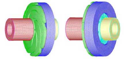
Figure 4. Single-stage flow channel mesh

，

3 u ^e p = -

К У р

y + = Р^Ур = p:'k PH yp where: P p p ; Wall friction coefficient “T = ^Tw /p ; Constant E and к are taken as 9.011 and 0.419.

• Multi-reference system model (MRF)

The flow in each section was solved in dynamic and a static double reference system. The rotating frame was fixed to the rotor with speed 2850 r/min, and the static frame was adopted in the inlet section, guide vane and outlet section. The connection surface between the two sub-regions is the interface. The coupling between the rotator and stator was simulated in Multiple Reference Frame (MRF).

III. Related issues of numerical simulation

Solution Setting: The standard k - e model, SIMPLE algorithm, second order upwind discrete difference equations were applied in the simulation. The residuals

convergence precision was set to be 10-4, and the others were solved by the default settings (without additional instructions, use this setting).

A.    Selection of grid number

Theoretically, with increase of the grid number, the solution errors caused by grid will gradually shrink, and even disappear. However, considering the configuration of the computer and computing time, the grid number can not be too much. In this paper, nine different grid numbers were divided, respectively shown in Table 2 and Fig.5. The size of the axial force with different grid numbers was compared, (the axial force do not include the gravity), and finally the appropriate grid number was selected.

TABLE II. The axial force with different grid numbers

Grid ( 10⁴ ) 13   19 26 35 45 51 76 95 130

F ( N )    471 475 490 500 503 493 493 495 507

0             50            100           150

Grid *104

Figure 5. Axial force – grid number curve

From Table 2, Fig.5, it can be seen that:

• a)    The axial force is relative small under less grid number, the. When the grid number reached 350 000, the difference of axial force is about 2.8%, tending to stable;

• b)    Taking computing time and coordination precision into account, the grid number of 450 000 meets the requirements.

B.    Selection of residual convergence precision

The solution of a steady-state problem usually can be obtained by large amounts of iterations and the convergence of the solution may be affected by many factors. A large number of computing units, the conservative relaxation factors and physical properties of complex flows are often the main reasons. Sometimes, it is difficult to determine whether you get the convergence solution.

In the iterative process, the convergence of solutions was monitored at all times, and ended when the specified accuracy was reached in the system. For there is no uniform standard, this section is empirical.

For the single-stage 200QJ20 type submersible pump model, its total grid number is 450 000, the residual convergence accuracy is set to 10-5. The axial force under different iteration number of the pump are shown in Table 3 and Fig.6, where when the iteration step number is 400, the residual convergence accuracy reaches 10-3; iteration step number 883, the residual convergence precision reaches 10-4; when the number of iteration step get to 2200, the residual convergence precision is close to 10-5.

Table III. The axial force under different iteration step number

Iteration step	100	200	300	400	500	600	700	800
F （ N ）	523	466	404	429	455	476	491	500
Iteration step	883	1000	1200	1400	1600	1800	2000	2200
F （ N ）	503	507	513	518	521	522	524	524

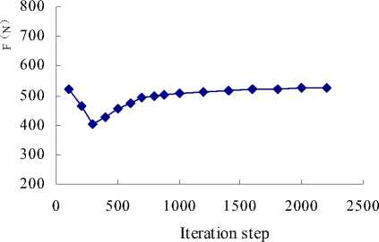
Figure 6. Axial force - the iteration step number curve

From Table 3, Fig.6 we can see:

• a)    Before the number of iterations step reaches 400, that is, the convergence precision of the residuals is less than 10^-3, axial force is very unstable and the discrete equation is not convergence.

• b)    When the number of iteration step is between the 400 and 883, that residual convergence precision between 10^-3 and 10^-4, the axial force increases, without stable trend.

• c)    After the number of iteration step reaches 883, residual convergence precision is over 10^-4, the axial force increases slightly and then tends to stable, and the residual convergence trend is slow. Taking the balance of solution precision and computing time into account, the convergence precision set to 10^-4.

C.    Turbulence model selection[5-6]

Turbulence appears in places where velocity fluctuates. Such volatility makes the exchange of momentum and energy between the fluid medium, and concentration changes. Because this fluctuation is small scale and has a high frequency, the direct simulation in the actual project calculation needs high requirements on the computer. In fact, instantaneous control equation may be uniform in time and space, or change the scale artificially, so the modified equations need less computing time.

However, the modified equations may contain the unknown variables, and the turbulence model needs to use the given variables to determine these variables.

Many turbulence models are provided in FLUENT, but a turbulence model is not universal for all problems. For different problems, the main reference points for choosing the model are as follows: whether the fluid is compressible, the establishment of a feasible issue, accuracy requirements, the computing capability, time limit and so on. The standard k-ε , RNG k-ε and standard k-ω and SST k-ω model were applied to calculate the axial force, shown in Table 4.

TABLE IV. Axial force under different models

Turbulence models	k - ε			k - ω
	Standard	RNG	Realizable	Standard	SST
F ( N )	503	514	524	520	526

In the table 4, the axial force obtained by the standard k - ε model is the smallest, but the axial force obtained by different models are almost the same, and difference between the maximum and minimum is 4.6%. In the iterative process, it’s fast to converge with the standard k - ε model; the computational time is much less than with other models. Therefore, the unified standard k - ε model was used in the simulation of single-stage 200QJ20 deep well pump.

D.    Algorithm Selection

The flow field solution of relevant issues has been briefly introduced in the previous section, so there’s no need a specific introduction, only for this model, SIMPLE, SIMPLEC and the PISO algorithm to compare the pump axial force the value respectively, as shown in table 5.

TABLE V. Axial force under different algorithms

Algorithms	SIMPLE	SIMPLEC	PISO
F ( N )	503	502	492

From Table 5, axial force obtained by using SIMPLEC algorithm and SIMPLE is almost the same, but only slightly difference with using PISO algorithm. Among them, it’s easy to converge and costs less computing time by using SIMPLEC. Therefore, the SIMPLEC algorithm was used in this simulation of a single-stage-type deep well submersible pumps.

E.    Roughness influence

The single-stage 200QJ20 deep well pump in this paper is composed of inlet section, impeller, guide vane and outlet section. Considering the actual situation, only the roughness of impeller and guide vane surface was set, and the roughness of inlet and outlet section was set to be zero. Roughness influence on the axial force is shown in Table 6.

TABLE VI. Axial Force under different roughness

Roughness ( mm )	0	0.05	0.1	0.15	0.2
F (N)	503	471	443	388	330

In table 6, the axial force decrease with the increase of roughness. It’s probably because hydraulic loss in the flow channel increases with the roughness increase, resulting to head reduces. The pressure at the same radius reduces, leading to axial force decrease. Considering the manufacture of the 200QJ20 type deep well pump, surface roughness value was set to 0.1mm

W ANALYSIS OF INTERNAL FLOW FIELD

Based on the above study, in this section we’ll do the numerical simulation of 200QJ20 type deep well pump, a total of 45 million meshes, residual convergence precision of 10^-4,using the standard model k - ε , SIMPLEC algorithm, impeller and guide vane surface roughness is 0.1. In order to facilitate comparison with the following experimental values, the import of impeller seal faces’ axial clearance is 0.3mm. Based on simulation results, we analyze the velocity and pressure distribution of the 200QJ20 type deep well pump.

• A. Velocity analysis

Do the whole level flow passage cross-section x = 0, as shown in Figure 7of the vector.

1 85^01 1 76e*01 1 66e*01 1 57e*01 1 48e*01 1 39e*01 1 30*01                   '    .'

• 1    21^01

1 11е*01 1 02^01 9 31e*00 8 39e*00 7 48^00 6 58e*00 5 64e*00 4 73e*00 381e*00 • -290*00    -

1 98**00^

1 06**00” '

1 40-01" "

• ( a ) Flow rate of the whole runner

  ( b ) Speed chart of amplified

  
  

cavity

— 988e*00

И 9 30*00

И 8 90e*00

Я 8 41e»00

6 94e*00

8 45e*00

590*00

1 5 47e*00

498e*00

4 4Be*00

4 00*00

3 51e*00

3 02H00

2 53^00

2 05^00

1 58e*00

1 07еЧЮ

5 77e-O1

8 6002

• ( c ) Distribution of turbulent Kinetic

• Figure 7 .    X=0 Vector section

As known from Fig.7 (a), the whole flow passage has no significant back flow and vortex; the velocity of the impeller outlet is to the maximum, but decreases gradually after the guide vane, which is in line with the actual situation. Since the impeller outlet miter, the exit velocity point to the rear cover, having no significant impact on the inner wall of the pump, we know that increasing the front cover diameter of the impeller does not increase the impact of the loss at the outlet of the impeller. Vortex forms in the guide vane inlet, indicating that guide vane inlet design has some certain problems, which needs to be further improved.

Fig.7 (b) for the velocity figure of the amplified cavity around the impeller, we can see the front cover cavity, liquid away from the cover side flowing inward ,and liquid near the cover side flowing outward, pointing to the impeller outlet, while the middle part of the cavity flow is slow. However, fluid flowing in the back cover cavity is chaotic, having no obvious regularity.

Fig.7 (c) for the distribution of turbulent kinetic energy of the whole level cross sections x = 0, we can see turbulent kinetic energy of the impeller inlet; outlet and guide vane inlet is large.

Fig. 8,Fig.9 for the relative velocity vector graph and distribution of turbulent kinetic energy of impeller, the middle cross section of guide vane, we can see:

• a)    Liquid velocity in the impeller has uniform distribution, no significant back flow and vortices, the performance of the overall symmetry is apparent. Large turbulent kinetic energy at the inlet, there is some impact, but not very obvious. A large turbulent kinetic energy in the impeller outlet, flow instability, to some extent by the inner wall of the pump.

• b)    The overall flow of the fluid in guide vane is stable, but the inlet has obvious vortex, turbulent kinetic energy is also great, while back flow at the outlet is not obvious.

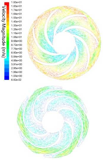
Figure 8 ． Relative velocity distributions in the impeller and guide vane

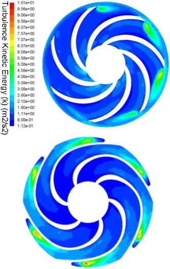
Figure 9 ． Distributions of turbulent energy on the cross-section of impeller and guide vane

• B. Pressure Analysis

Fig.10 shows the total pressure cloud map of overall level flow passage, total pressure i.e. total energy, we can see the total energy gradually increased from the impeller inlet to outlet, and to the maximum at the end of the blade near the front cover, then the energy gradually decreased along the guide vane flow passage and stabilized at the outlet. Fig.11shows the static cloud graph of impeller, the middle cross section of guide vane, we can see static pressure are evenly spaced from impeller inlet to the outlet, the working side pressure is to the maximum at the end of blade, you can see the minimum pressure in the back of the blade near the inlet, which is negative, cavitations occurs most likely in this region. Static pressure gradually increased from guide vane inlet to outlet, indicating that the kinetic energy gradually converted to pressure energy.

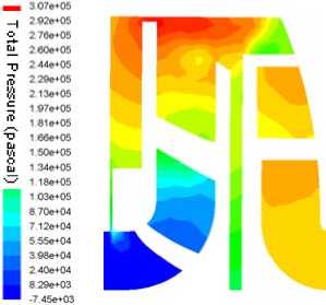
Figure 10 ． Distributions of rated flow turbulent energy

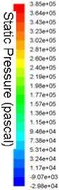
Figure 11. Static pressure distributions on the cross-section of impeller and guide vane

V RESULTS ANALYSIS AND AXIAL FORCE CALCULATION

A. Axial force calculation

Considering the axial force characteristics of numerical simulation of deep well pump, the composition of the axial force is divided as follows.

• a)    The axial force F ₁ of the outer surface of impeller front shroud;

• b)    The axial force F ₂ of the outer surface of impeller back shroud;

• c)    The axial force F ₃ of the seal face axial clearance of impeller inlet;

• d)    The axial force F ₄ of front surface and back surface of impeller blades;

• e)    The axial force F ₅ of cutting impeller outlet;

• f)    The axial force F ₆ of impeller inner channel surface;

• g)    The axial force F ₇ of pump shaft, which is an important component to the axial force in a deep well pump; the more stages are, the larger its value is;

• h)    Gravity of impeller and the shaft F ₈ , which does not exist in the horizontal pump. In this study 200QJ20 type deep well pump is a vertical pump, F8 = 30 N .

The axial force of impeller corresponds to the sum of the six forces, F i = F + F 2 + F ₃ + F 4 + F 5 + F 6 ; and the axial force of the whole pump is the sum of the eight forces.

Fig.12 shows at nominal operating condition Q = 20 m³/h , the static pressure distribution of impeller front and back shroud, the seal face axial clearance of impeller inlet , cutting impeller outlet, front surface and back surface of impeller blade and impeller inner channel surface.

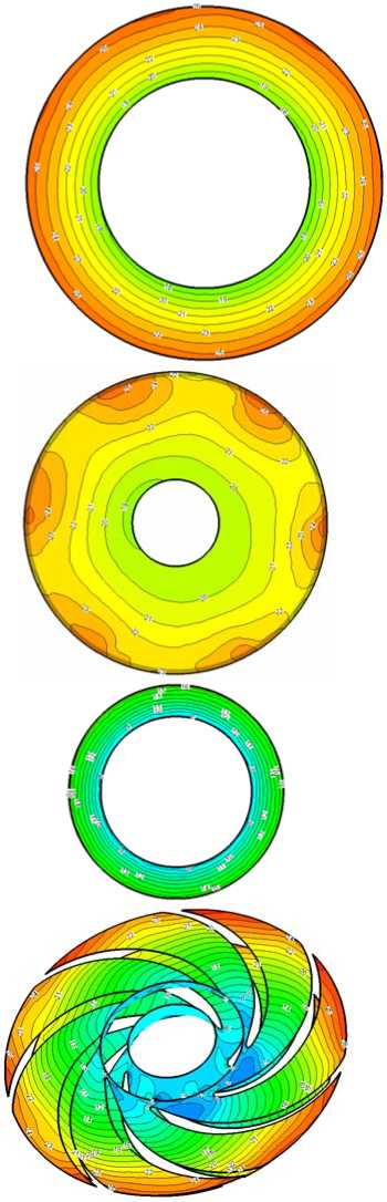
TABLE VII. PREDICTED AXIAL FORCE

(i n ’ /h) F i ⁽ N ) F 2 ⁽N ) F 3 ⁽ N ) F 4 ⁽ N ) F'"' N ) F6^(ЮF 7 ' N F8^(ЮF ^(ЮF ^(Ю

8	-1743	2017	-167	47	99	495	140	30	748	918
12	-1740	1976	-160	62	96	474	137	30	708	875
16	-1726	1919	-157	76	94	451	135	30	657	822
20	-1709	1848	-157	89	93	427	131	30	591	752
24	-1686	1757	-158	100	91	400	125	30	504	659
28	-1654	1649	-160	111	88	370	116	30	404	550
32	-1614	1531	-161	121	84	337	104	30	298	432

Figure 12 . The static pressure distribution on impeller surface

The six axial forces can be obtained by Fluent post-processing directly, and the axial force F ₇ can be obtained by integral of the static pressure of pump outlet, and gravity F ₈ is given. So the total axial force of 200QJ20 type deep well pump can be obtained.

Table 7 shows the predicted axial force value of full conditions, where "-" means that the direction of the force points to the pump outlet.

From the analysis of the axial force components at rated operating conditions in table 7, it can be seen that:

• a)    The axial force F ₁ and the axial force F ₃ are negative, which means that point the direction of pump outlet, the other components point to the inlet.

• b)    The axial force of the external surface, F ₁ + F ₂ + F ₃ + F ₅ = 111N, about 15% of the total axial force. The proportion is small, this is because impeller outlet is oblique, reducing the area of impeller back shroud.

• c)    The axial force of impeller inner channel surface (including the front blade, back blade), that is, F ₄ + F ₆ = 516N, 70% of the total axial force, this force is difficult to calculate by the empirical formula accurately,

but it is the most important part of axial force in 200QJ20 type deep well pump.

• d)    Axial force F ₇ of shaft end suffered approximately 20% of the total axial force F ; the force increases more with more stages and higher head.

From the analysis of the axial force of the whole conditions, we can see:

• a)    With the flow increases, the pump head decreases, F , F 2 , F 5 , F 6 and F 7 decrease, but F 4 increases.

• b)    The axial force F ₃ of the seal face axial clearance of impeller inlet F ₃ is less affected by flow changes, and the reasons need to be further studied.

• c)    With the increased flow, the axial force of impeller’s out surface are 206,172,130,75,4, -77,-160N, which shows that the force decreases gradually, and then increased gradually after the direction changes.

• d)    With the flow increases, the axial force F i and F also decrease sharply, which indicates that the flow have a significant influence on F i and F .

• 4 THE EXPERIMENTAL STUDY OF STUDY OF 200J20-TYPE DEEP WELL PUMP

A. The axial thrust test of the seal face axial clearance ( 0.3 mm) of impeller inlet

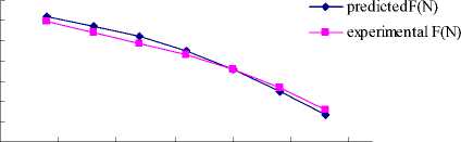
The axial force test device of the 200QJ20 type submersible pump was designed, with simple structure and high precision. In order to investigate the influence caused by the seal face axial clearance of impeller inlet, the axial force was measured. The axial force under multi-conditions was measured respectively, shown in Table 8 and Fig. 13. The axial force points to the direction of impeller inlet.

4       9      14      19      24      29      34

Q(m3/h)

Figure 13. The predictive and test value of F-Q curve

TABLEVIII. THE PREDICTED AND TEST AXIAL FORCE

Q ( m3/h)	Predicted F (N)	Test F (N)	Error
8	918	894	2.7%
12	875	840	4.2%
16	822	784	4.9%
20	752	730	3.0%
24	659	657	0.3%
28	550	567	3.0%
32	432	459	5.9%

From Table 8 and Fig. 13, we can see:

• a)    For the four stages 200QJ20 type deep well pump, the single-stage axial force was converted according to the experimental data. The weight of the submersible motor rotor is10kg, and the experimental axial force in the table lists contains no the rotor weight. So the test value listed in the table is the axial force of single-stage 200QJ20 type deep well pump, which is the sum of the axial force of the pump shaft, impeller gravity, impeller and shaft.

• b)    With the flow increases, predicted and test values of the axial force reduce gradually. The F-Q curve trend of each other is generally the same, and there is no great fluctuation at the small and large flow, which indicates that the predicted axial forces under fully working conditions are accurate.

• c)    Comparing the predicted values with test values, the maximum error is 5.9% and the minimum error 0.3% at full operating conditions. Hence the predicted axial thrust by using numerical simulation is feasible.

Ⅶ TEST OF AXIAL FORCE WHEN IMPELLER

INLET SEAL AXIAL CLEARANCE IS ZERO

As to the structural constraints of the measurement device, the impeller seal axial clearance of inlet is zero in the experiment is difficult to achieve, therefore, by repeatedly adjusting column load cell axial clearance is to the minimum, as close to zero.

Impeller inlet seal axial clearance is zero in the numerical simulation is very easy to implement, and reduces the difficulty of meshing. But there is a problem, because the axial clearance is zero, the impeller inlet seal face has no liquid, and the suffered axial force can not be obtained directly.

The shape of seal face of impeller inlet is respectively to the radius of the impeller inlet and the radius of seal ring, assuming the pressure in the seal surface is trapezoidal distribution, the average pressure obtained from post processing inner and outer ring by Fluent, so axial force of seals can be obtained by integration.

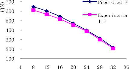
All conditions are given below the predicted and test values, are respectively shown in Table 9 and Figure 14.

TABLE К . PREDICTIVE AND EXPERIMENTAL VALUE OF

AXIAL FORCE

Q ( m3/h)	Predicted F (N)	Experimental F (N)	Error
8	647	612	5.7%
12	602	567	6.2%
16	544	517	5.2%
20	472	454	4.0%
24	399	389	2.6%
28	315	302	4.3%
32	219	208	5.3%

Q ( m³/h )

Figure 14 ． Predictive and experimental value of F － Q

Table 9, Fig.14 shows:

• a)    With the flow increases, the predicted and experimental axial force values are gradually reduced, the F-Q curve is also broadly consistent with the trend, and the small flow and large has none of greater volatility, indicating that all conditions of the axial force predicted values is accurate.

• b)    Under all conditions, predictive values compared with the experimental values of maximum error 6.2%, minimum error 2.6%, the average error is 4.8%, deviation is slightly larger when the axial clearance is 0.3mm..

• c)    At present, using numerical simulation to predict the performance of the pump, the large flow and small flow deviations are large; generally no longer have reference value, while the axial force prediction has no such problems.

The reasons may be:

• (a)    When predict the efficiency and the pump head, the impeller of the liquid flow, the guide vane or vortex chamber fluid flow and at the junction of the impeller and guide vane or vortex chamber the liquid flow is critical, that predictive values are determined by overall level flow passage.

• (b)    While the impeller axial force is mainly determined by fluid flow in the impeller, guide vane or vortex chamber has little effect on liquid flow, and the impeller axial force accounted for about 80%, so that prediction of the axial force is more reliable than the performance prediction.

W CONCLUSION

The axial force issues have been studied by many experts in recent years, but it is difficult to calculate the size of the axial force accurately due to complexity of the inner flow field. On this basis, the paper carried out the following research:

• a)    In order to enhance the numerical simulation precision, the influence caused by entity modeling, meshing, residuals precision, turbulence model, and numerical solution method was investigated. Then the best scheme was selected to simulate the submersible pump.

• b)    The estimation of axial force in submersible pump based on CFD was brought forward for the first time. The 200QJ20 type submersible pump was

simulated in Fluent, obtaining pressure distribution of flow field and the axial thrust value.

• c)    The axial thrust test device of the 200QJ20 type submersible pump was designed, with simple structure and high precision. In order to investigate the influence caused by the seal face axial clearance of impeller inlet, the axial thrust values were measured at the clearance of 0.3 millimeter. Comparing the estimating values with testing values, the maximum error is 5.9% and the minimum error 0.3% at full operating conditions. Hence the predicted axial thrust by using numerical simulation is feasible.