The fast algorithm of intermediate perspectives reconstruction on a stereopair

One of the up-to-date trends of video information ideas is supposed to be the task of presenting dimensional data. Due to this, devices which are able to produce volumetric images (multiperspective monitors, projection systems) are becoming more and more widespread. For the proper functioning of these devices it is necessary to obtain a certain number of perspectives of the reproduced scene; the number of which is defined by a certain task. For instance, for watching videos 4–6 perspectives are usually enough for comfort. For serious applications such as 3D-tomography and radiography, graphical work stations CAD/CAM, the representation of presented settings (control tower, search, and rescue services), etc, one could require from 40 to 150 perspectives. There are some special devices providing from 2 (stereo-video cameras) to 8 perspective settings. 8 perspectives video cameras were used in a prototype multiperspective NIKFI television system, and it is quite difficult to imagine a video camera with a large number of perspectives.

Equally difficult is considered the recording and transmitting of such a signal through connecting channels. Consequently, there is a need to reconstruct a required number of perspectives – i.e. images which have been obtained with the help of a similar camera, if it had an intermediate position between cameras used in stereo filming. The majority of algorithms solve this problem on two levels: searching for the corresponding points, i.e. points at the images fitting to the same spot of a three dimensional space, and the approximation of intermediate perspectives on the basis of the reveled appropriate points. Usually, if all the corresponding points, found at the approximation of the intermediate perspectives cause no difficulties the primarily object of the intermediate perspective reconstruction is the search for corresponding points. As an example let us examine the functioning of a simple stereovision algorithm. It consists out of several steps:

• 1.    We have selected the first (upper) epipolar line as a current line.

• 2.    For the current epipolar line we have selected the pixel most left of the current pixel.

• 3.    We have matched the current pixel of the left image to every pixel of the right image.

• 4.    We have selected the most similar pixel from the right image and wrote it in the array of the corresponding pixels. The array of corresponding pixels represents a 2D integer-valued array; the index elements of which are the

• 5.    If the current pixel is not the last in the active row then the following pixel is getting the current pixel and the algorithm goes to item 3. Otherwise, to item 6.

• 6.    If the active epipolar line is not the last line, then the following epipolar line becomes active and goes to item 2. Otherwise the algorithm stops functioning.

positions of the pixels on the left image and the meanings of the elements – are the positions of the corresponding pixels of the right image.

The functioning of a simple stereovision algorithm is presented as a logical diagram (as shown in fig. 1). The result of the algorithm functioning is an array of corresponding pixels. Then, using this array one can build a depth card or reconstruct the intermediate perspectives, i. e. images which could be obtained with a similar camera in case it took intermediate positions between the cameras, used in stereo filming.

The reconstruction of intermediate views according to the A. A. Lukianitsa method. Setting the task. Suppose we have a stereo pair – i.e. two images of the same setting fixed done with a stereo camera. Let’s mark the image taken by the left camera, with letter L , and the image of the right camera – with letter R . Let’s introduce the orthogonal coordinate system coordinated with the cameras: we direct axis X to the right, through the image centers, axis Y – downwards along the vertical image axis and axis Z adds them to the right three. The starting point of the coordinate shall be chosen in such a way that the images are in the Oxy plane, and image centers are symmetrical according to plane Oyz (fig. 2). This setting is registered by two cameras: L and R . We need to build an intermediate perspective M .

Say the center of the left image in the chosen coordinate system has the coordinates ( x L ,0 ,0), and the center of the right is – ( x_R ,0 ,0). The task is that an image should be built in the plane Oxy with its center in a point ( x_M , 0, 0), closely situated to the image which was received by the camera the optical axis of which would pass through point ( x M , 0, 0). The suggested method consists of two levels:

• –    the location of the corresponding points on the left and the right images;

  – the approximation of the intermediate image on the base of conjugated points and the filling of the fields for which the correspondence is not single-digit [1; 2].

The search algorithm for corresponding points. Say every image contained K × N pixels on the horizontal and vertical lines correspondingly. The task of finding the conjugated points is the following: for every pixel of the left image Lki, k = 1, …, K, i = 1, …, N. We need to find pixel Rkj, j = 1, …, N at the right image corresponding with the same point of the registered settings.

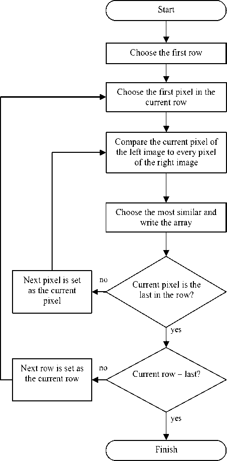
Fig. 1. The logical diagram of the stereovision functioning for a simple algorithm

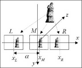
Fig. 2. Geometry of stereo filming

Suppose the cameras were fixed at the same horizontal line and have the same gain constant. Then the horizontal lines of the photo detectors coincide with the epipolar lines; that’s why the conjugated point should be situated on the lines with the same number. This allows us to write down the following expression for calculation the epipolar lines:

L(k,i) ≈ R(k, j + ∆j), where Δj – is a shift, depending on the pixel number.

The finding of the corresponding points consists in the calculation of a displacement for all pixels. Further, for simplicity we shall omit the first index, because it has the same value for the compared images, and state that the process described below is executed for each pair of corresponding lines in the left and right images. To find expedient candidates for corresponding points we should compare some areas Ω in the environment of these pixels. It essentially increases the stability of the algorithm. Indeed, there may be differences in the images with a similar section of the scene under different angles, because of the mutual position of light sources and scenic elements. Besides, some areas can be visible for one camera and are invisible for another.

Let the compared area Ω have the following sizes k × n , then in the environment of the j -th pixel on the right image we should scan a bigger sized area: m × l , m ≥ k , l >  n . The distance function d ( i , j ) is calculated during the scanning process. This function characterizes the proximity of images in area Ω i of pixel L ( i ) and in area Ω j of pixel R ( j ). The distance function is usually taken as a sum of differences for corresponding pixels intensities from Ω i and Ω j :

k /2 n /2

d ( i , j ) = Z Z L ( k + m , i + 1 ) - R ( k + m , j + 1 )|, m =- k / n 1 =- n /2

or as the comparing of the images from Ω i and Ω j gradients.

Practically, it is better to use a combination of these methods, because they have various efficiency for different types of images. Often, various researchers use a method of intensity comparison; however; when image processing with homogeneous vast objects, for example, a house wall, this method leads to the appearance of a plateau for function d ( i , j ) that complicates a selection of corresponding points. In this case the gradient difference allows the considering of “thinner” image details.

To select the corresponding points from all possible pretenders we should meet two conditions. First of all, it’s obvious that the index numbers of the corresponding points should minimize the total difference of the compared areas on the left and right images. Secondly, the offset value cannot decrease in the process of index j increase, i. e. Δ j ≥ Δ j –1 . This condition follows from the geometric properties of the stereo pair. Th next algorithm based on the dynamic programming method is offered to satisfy these conditions.

Let’s introduce two accessory functions: real ψ and integer P . The first of these is necessary for the accumulation of total differences for compared areas. The second is reserved for the storage of appropriate indexes.

The dynamic programming algorithm consists of three steps:

• a)    Initialization:

• V ( i ,1) = d ( i ,1), i = 1,..., N ;

P ( i ,1) = i ,        i = 1,..., N .

• b)    Inductive passage:

V ( i , j ) = min V ( k , j - 1) + d ( i , j ), i = 2,..., N , j = 1,..., N , 1 < k <  i

P ( i , j ) = argmin v ( k , j - 1), i = 2,..,N , j = 1,..., N .

1 < k < i

• c)    Reverse move:

J ( N ) = arg min y ( i , N ),

1 < i <  N

J ( j ) = P ( J ( j + 1), j + 1), j = N - 1,...,1.

The array of indexes for corresponding points J at which for any pixel of the left image L ( i ) the corresponding pixel of the right image is described as R ( J ( i )) will be constructed in result. The dynamic programming algorithm is presented in fig. 3.

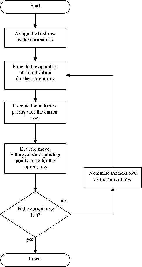
Fig. 3. The dynamic programming algorithm

This algorithm executes image processing line-byline; this allows parallelizing calculations. It considerably speeds up stereo reconstruction procedures, but a consequence of progressive processing may be the effect of “combing”. Unfortunately this algorithm does not offer any methods of reducing these effects.

Let’s consider each step of the presented algorithm in detail. The initialization procedure serves for the definition of initial values of functions ψ and P . Function ψ is calculated as d function between the first pixel of the left image in the current line and each pixel of the right image in the current line. P function is calculated as pixel indexes of the right image.

The next step of the dynamic programming algorithm is the inductive passage. Here calculated are the subsequent values of functions ψ and P . Function ψ accumulates the total values of the compared areas. The total difference accumulation of compared areas increases the accuracy of finding corresponding points.

The last step of the dynamic programming algorithm is a reverse move. At this step the corresponding array point J is filled. The pixels of the right image, which have a minimal difference between each other, are selected as corresponding points for the pixels on the left image.

Intermediate view approximation

Let’s introduce parameter a = xM—xL- , which

XM — XR characterizes the relative degree of proximity for the reestablished view on the left image. Further for all values of i = 1,…,N, j = 1,…,N we will calculate:

k = [α j + (1 – α) J ( j )], M ( i , k ) = α L ( i , j ) + (1 – α) R ( i , J ( j )).

As we can see from these correlations some points of the intermediate view can be unfilled. This happens because the corresponding fragments of the threedimensional object are visible for one camera, but invisible for the other. Let it be that in the reconstructed image in any i -th row pixels j 0 , …, j 0 + m are unfilled. There are two cases:

– if J ( j ₀ – 1) = J ( j ₀ + m + 1) then these pixels are visible only for the left camera and they are filled by proper values from the left image:

M ( i , j ) = L ( i , j ), j = j 0 , …, j 0 + m ;

– if J ( j 0 – 1) <  J ( j 0 + m + 1) then these pixels are visible only for the right camera and they are filled by respective values from the right image:

M ( i , j ) = L ( i , J ( j )), j = j 0 , …, j 0 + m .

Increasing the speed of the algorithm. Though the speed of this algorithm is high enough, it can be insufficient for the solution of some tasks. Consequently, it’s necessary to find a way of increasing the presented algorithm speed.

As a rule, in all stereo algorithms the CPU time for most of the part is occupied by the calculation of the distance function for the row pixels. To minimize the time spent on the distance function calculation it is necessary to simplify the function or decrease the quantity of pixels for which it is calculated. One of the possible variants consists in decreasing the size of the frame around the selected pixels but this does not always give good results, and is not applicable for all images.

Apparently, from the aforesaid, the simplification of the distance function is not possible; therefore, it is necessary to reduce the number of computations for this function. The improvement of the discussed algorithm is linked with the introduction of an additional variable: maximal disparity D max . Maximal disparity is the maximal difference between the offset of a point in threedimensional space on the left and right images. This variable is set by the user for each stereo pair. The value of this variable can be calculated if the location of the cameras and the distance from the stereo photography plane to the maximal distant object of the scene is known. Let’s rewrite the expressions used on steps of the initialization, the inductive passage, and the reverse move; given the setting of maximum disparity in the following form:

• 1.    Initialization:

• V ( i ,1) = d ( i ,1), i = 1,..., N ;

• 2.    Inductive passage:

• 3.    Reverse move:

P ( i ,1) = i ,         i = 1,..., N .

^ ( i , j ) = min y ( k , j - 1) + d ( i , j ), i = 2, D max - ^k - i

N , j = 1,..., N ,

P ( i , j ) = argmin v ( k , j — 1), i = 2,..., N , j = 1,..., N . ^ max ^{- k -} i

J ( N ) = arg min ^ ( i , N ),

D max ^- i ^- N

J ( j ) = P ( J ( j + 1), j + 1), j = N - 1,...,1.

In result of the entered changes, the speed of the algorithm considerably increases because now there is no necessity to compute the value of the distance function for each pair of pixels in a row. The presented algorithms were realized in C ++ language. The realized experimental algorithms have been carried out (sce table). The time for locating corresponding points of one line has been measured. The distinctions in the results of algorithm operating have been evaluated. Comparison has been carried out on a test stereo pair with a 10 pixel width (fig. 4).

From table it is apparent that the modified algorithm has a higher speed. However, the quantity metric of truly defined corresponding pixels worsens by 2–6 % in comparison to A. A. Lukjanitsy’s base algorithm [2].

In this article the stereo reconstruction algorithm of Lukianitsa A. A. had been overlooked. The speed of this algorithm was also estimated. Modifications, which increase the speed of this algorithm, were offered. The modified algorithm was realized in high-level programming language ( C ++). In result of the conducted experiments, the operation speed of the modified algorithm at insignificant deterioration of stereo reconstruction was registered.