The Forecast of Jute Export in Bangladesh for Optimal Smoothing Constants

Автор: Md N. Dhali, Anirban Biswas, Al-Amin, Md M. Hasan, Nandita Barman, Md K. Ali

Журнал: International Journal of Mathematical Sciences and Computing @ijmsc

Статья в выпуске: 2 vol.9, 2023 года.

Бесплатный доступ

Forecasting is estimating the magnitude of uncertain future events and provides different results with different supposition. In order to identify the core data pattern of jute bale requirements for yarn production, we examined 10 years' worth of data from Jute Yarn/Twin that were shipped by their member mills Limited. Exponential smoothing and Holt’s methods are commonly used to forecast this output because it provides an adequate result. Selecting the right smoothing constant value is essential for reducing predicting errors. In this work, we created a method for choosing the smoothing constant's ideal value to reduce study errors measured by the mean square error (MSE), mean absolute deviation (MAD), and mean square percent error (MAPE). At the contrary, we discuss research finding result and future possibility so that Jute Mills Limited and similar companies may execute forecasting smoothly and develop the expertise level of the procurement system to stay competitive in the worldwide market.

Еще

Jute Export, Exponential Smoothing Method, Holt’s Method, Smoothing Constants

Короткий адрес: https://sciup.org/15019051

IDR: 15019051 | DOI: 10.5815/ijmsc.2023.02.04

Текст научной статьи The Forecast of Jute Export in Bangladesh for Optimal Smoothing Constants

1. Introduction
2. Exponential Smoothing Method and Holt’s Method

Jute has long been significant to Bangladesh's economy. Exporting raw jute, jute products, and jute-based arts and crafts allowed Bangladesh to make significant amounts of foreign currency. It was given the nickname "Golden Fibre of

Bangladesh" for this reason. Bangladesh has remained to be the world's greatest producer of high-quality jute due to its agroclimatic conditions. It supports the livelihoods of millions of industrial employees and farmers. Additionally, it has been a significant contributor to export revenue. It plays a significant role in creating our national budget as well. Jute and jute goods therefore have a growing potential as natural eco-friendly products. Bangladeshi producers and exporters are currently concentrating on a variety of jute goods due to rising global demand. Therefore, it is essential to know the anticipated export volume in order to create an annual budget for the following year.

Holt's approach is straightforward and can produce accurate forecasting results on par with those of more sophisticated methods. This approach is common, easy to use, and often effective in real-world settings. Two smoothing constants have been utilized in this method to evaluate the forecast value and smooth the forecast value. So, determining the ideal smoothing constant value is crucial for producing better forecasts. Our project's goal is to forecast the export of jute using the exponential smoothing approach and Holt's method for selecting the best smoothing constants.

Jute's significance to Bangladesh's economy is well known and doesn't need to be emphasized. Roughly 10% of all jobs in the nation are related to jute cultivation, trading, and industry, which also makes up about 12% of the GDP. Consequently, it is crucial to forecast jute's revenue. The primary objective of this study is to anticipate future jute exports.

A study is developed to forecast the foreign remittances in Bangladesh for optimal smoothing constants [1]. A suitable forecasting method is acquired for the recently established biscuit industry in Bangladesh [2]. A thorough process was utilized to assess the ideal smoothing constant values for the Holt's method, the Holt-Winter seasonal multiplicative method, and the Exponential smoothing method [4, 5]. MAD and MSE are calculated for a specific problem using various smoothing constant values, and the best smoothing constants are chosen by choosing the smallest values of MAD and MSE [6]. It is attempted to analyze the projections for solar irradiance and load demand using single smoothing forecasting algorithms [8]. Bermudez et al. had been worked improving demand forecasting accuracy using nonlinear programming software [11]. In order to determine the best smoothing constants, a suitable quantitative forecasting method for predicting private car demand in the city of Dhaka is studied [13].

The simplest form of exponential smoothing is given by the accompanying formula:

The forecast for the t + к period with the basis of t period is

^F t,k = ^a^ t + ^к * ⁽1 - ^a)F t+1

Where,

Ft+1=Forecast for period (t + 1)

^kt, к = Forecast for period (t + к)

On the other hand, a well-liked smoothing technique for trend-based data forecasting is Holt's Method. Two parameters are used in Holt's method: one for trend smoothing equation and the other for overall smoothing. In that instance, a variety of methods known as "Holt's method" have been created to address the complexity of predicting errors.

It should be emphasized that Holt's technique works effectively in situations when there is merely trend and no seasonality.

Here, the time series shows a trend, and the level variable must also be calculated along with the trend (slope). At the conclusion of time t, the forecast for the t + к period is given by

F t+к = Ц + к *T t

Here, ^L- is the estimate of level made at the end of period t and is given by

kt = °^t + (1 - a)Ft

T_t is the estimate of trend at the end of period f and is given by

T t =V(L t -L t-i ) + (1-P)T t-i

P is also a smoothing constant between 0 and 1 and plays a role similar to that of a .
3. Jute Export Investigation

Small values of aand p once more imply that estimations of the level L_t and trend T_t variables do not deviate much from one another. Any change, in the context of the new need, is minor. To begin the series of forecasts using this method, estimation of the initial level component and the initial trend component is necessary.

Initialization:

The initial estimated base label L₀ is assumed from the last period observation and initial trend T₀ is the average monthly or weekly change.

L₀ = Last period’s observation

T₀ = Average monthly or weekly increase

In Bangladesh, BJMA figure included their Jute whose value Tk. (Crore) exported by their member mills before last ten years. Actual values of jutes are also given. We have to forecast values for next ten years.

Table 1. Jute exports in Bangladesh for different years

Year	2010	2011	2012	2013	2014	2015	2016	2017	2018	2019
Exports (in Crore BDT)	95.79	95.79	95.79	95.79	95.79	95.79	95.79	95.79	95.79	95.79

The jute exports from Bangladesh in various years are shown in Table 1. Holt's approach must first be used to initialize the estimated base label and trend before evaluating the forecast value.

For simple Exponential smoothing method:

Initialization:

In order to use the exponential smoothing method to solve the given problem, we must first initialize the predicted value.

For smoothing constant α

Let, the initial forecast F 1 = 95.79

Now, a particular value of a determine whether MAD, MSE, and MAPE provide the least value by computing MAD, MSE, and MAPE.

The process is shown by the following Table 2

Constant(α)	MAD	MSE	MAPE
0.05	254.7576	120264.25	51.7508
0.1	227.3624	97682.087	46.9953
0.15	218.703	83022.229	48.0278
0.2	210.3566	73197.247	48.637
0.25	201.1029	66306.892	48.51
0.3	191.297	61200.0195	47.8199
0.35	187.933	57190.9803	47.939
0.4	185.072	53878.464	47.852
0.45	181.328	51031.425	47.3655
0.5	176.947	48518.381	46.5725
0.55	172.124	46264.366	45.547
0.6	167.003	44225.264	44.35
0.65	161.696	42372.897	43.025
0.7	156.287	40686.663	41.611
0.75	150.8394	39149.078	40.135
0.8	146.394	37743.625	38.936
0.85	144.842	36453.913	38.619
0.9	143.183	35263.562	38.242
0.95	141.396	34156.477	37.802

Table 2 demonstrates that the minimal values for the smoothing constants for MAD, MSE, and MAPE are all given by these functions.

Table 3 below displays lower values of MAD, MSE, and MAPE along with related smoothing constant values.

Table 3. Finding optimal values of smoothing constants a

Criteria	Minimum value	value of a
Mean Absolute Deviation (MAD)	141.396	0.95
Mean Squared Error (MSE)	34156.477	0.95
Mean Absolute Per. Error (MAPE)	37.802	0.95

According to Table 3, MAD, MSE, and MAPE all provide the least value of the smoothing constants is a = 0.95; as a result, a = 0.95 is the ideal value for the smoothing constants.

The forecast of next ten years BJMA figure included their Jute whose value Tk. (Crore) exported are in below:

Table 4. Forecast values for optimal smoothing constants a = 0.95

Years (t)	F_t(B.D in Crore)
2020	312.7606
2021	331.2386
2022	346.8766
2023	362.5147
2024	378.1527
2025	393.7908
2026	409.4288
2027	425.0669
2028	440.70495
2029	456.343

From Table 4, we get the forecast value for the next ten years. Using Exponential smoothing method the forecast value for the optimal smoothing constants a = 0.95 at the 2029^th year is 456.343

The comparison between the actual value and the matching predicted value for the best smoothing constants is shown in the accompanying Figure.

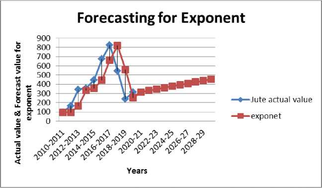
Fig. 1. Comparison of actual value and forecast value (Exponential smoothing method)

We employ the exponential smoothing method to resolve the stated issue. We obtain the ideal smoothing constants a = 0.95 for the exponential smoothing approach, and the predicted value for the year 2029 is 456.343. The worth of jutes over the next ten years is rising daily.

For Holt’s method:

Holt's approach must first be used to initialize the estimated base label and trend before it can be used to solve the presented problem.

Initialization:

Let the initial estimated base be L₀

And the initial estimated trend be T0

L₀ = Last year’s observation =315.75

T₀ = Average yearly increase

(165.9 - 95.79) + (344.67 - 165.9) + (358.8 - 344.67) + ••• + (315.75 - 240)--------------;----------------------|------------------------------------ = 24.44

Now that we know a specific value of a, we can compute MAD, MSE, and MAPE for the various values of /?. By continuing this process, we obtain MAD, MSE, and MAPE and determine whether MAD, MSE, and MAPE yield the minimum value by fixing a specific value of /? and altering the values of a. The process is displayed in Table 5 below.

constant (a)	constant (/?))	MAD	MSE	MAPE
0.1	0.01	142.4958	42666.0506	59.1403
	0.2	151.0114	46121.567	60.2124
	0.5	166.5762	52497.885	63.3641
	0.7	175.46872	56999.6292	65.5459
	0.9	183.1673	61620.2093	67.7231
0.2	0.1	159.9506	48064.8078	62.8965
	0.2	168.2365	51543.0554	64.7703
	0.5	193.5085	63198.9175	71.3858
	0.7	209.1221	71809.9387	75.9637
	0.9	222.6809	80929.426	80.2135
0.3	0.1	172.0545	50604.4	65.9326
	0.2	182.2177	55244.9916	68.5216
	0.5	208.6629	70713.473	76.2004
	0.7	220.5254	81046.546	80.1415
	0.9	226.7617	89823.716	82.5859
0.4	0.1	177.3662	51865.9991	67.1839
	0.2	187.282	57128.2936	69.8666
	0.5	207.1197	72820.3964	76.0456
	0.7	210.3424	80338.0392	77.5384
	0.9	206.1031	83631.9002	76.7823
0.5	0.1	177.1946	51867.1236	66.8143
	0.2	185.4035	57097.6731	69.0968
	0.5	195.1967	69817.73887	72.3832
	0.7	191.6121	72892.6994	72.1932
	0.9	184.5199	71480.275	71.6687
0.6	0.1	173.0571	50798.2101	65.1662
	0.2	178.841	55498.7426	66.7565
	0.5	182.8472	64219.6071	69.3849
	0.7	177.2348	64151.8114	69.4031
	0.9	167.5786	61224.1997	67.8178
0.7	0.1	166.2499	48968.2341	62.587
	0.2	170.7466	52909.075	64.1531
	0.5	172.3633	58239.9146	67.4445
	0.7	164.1373	56924.2658	66.449
	0.9	163.039903	54571.0965	66.6894
0.8	0.1	160.9702	46680.153	61.3271
	0.2	165.5721	49844.5492	63.6221
	0.5	161.9576	52892.0871	65.2252
	0.7	159.4802	51518.8331	65.5822
	0.9	161.2461	50267.4504	66.4972
0.9	0.1	156.644	44164.437	60.8898
	0.2	159.4345	46644.346	62.6696
	0.5	158.8293	48341.1907	64.8978
	0.7	157.3516	47344.9559	65.3161
	0.9	160.4931	46968.3248	65.9253
0.95	0.01	149.5513	40220.698	58.4114
	0.02	150.1632	40533.118	58.6695
	0.03	150.753	40843.153	58.924

Criteria	Minimum value	value of a	value of /?
Mean Absolute Deviation (MAD)	142.4958	0.1	0.01
Mean Squared Error (MSE)	40220.698	0.95	0.01
Mean Absolute Per. Error (MAPE)	58.4114	0.95	0.01

From Table 6, we see that, MAD, MSE & MAPE both give the minimum value for the value of smoothing constants a = 0.95 & /? = 0.01; therefore, a = 0.95 & /? = 0.01 are the optimal value of smoothing constants.

As shown in Table 6, MAD, MSE, and MAPE all provide the minimal value for the value of the smoothing constants a = 0.95 & /? = 0.01; as a result, a = 0.95 & /? = 0.01 are the ideal value for the smoothing constants.

The forecast of next ten years BJMA figure included their Jute whose value Tk. (Crore) exported are in below:

Years (t)	f^B.D in Crore)
2020-21	335.9068
2021-22	357.9046
2022-23	379.9024
2023-24	401.9002
2024-25	423.898
2025-26	445.8958
2026-27	467.8936
2027-28	489.8914
2028-29	511.8892
2029-30	533.887

The comparison between the actual value and the matching predicted value for the best smoothing constants is shown in the accompanying Figure.

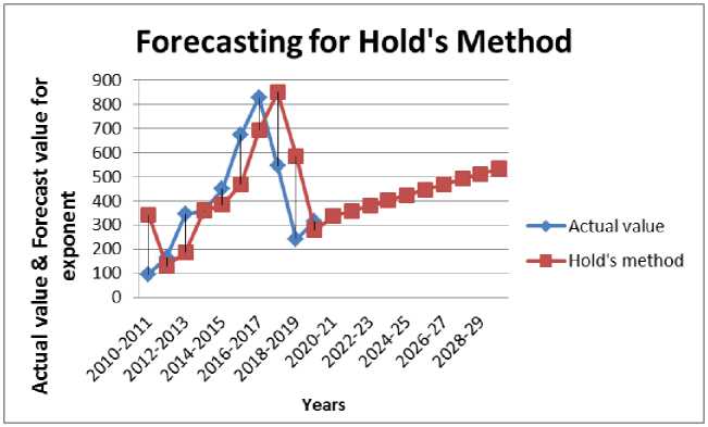
Fig. 2. Comparison of actual value and forecast value (Holt’s Method)

4. Conclusion

There are numerous forecasting methods now in use. In this research, we developed a method for choosing the best smoothing constants for the Holt's approach and the exponential smoothing method. In order to smooth the forecast accuracy, we include two constants. By providing an actual case, we portrayed the selection process. In order to forecast the value of jute shipped from Bangladesh, it was necessary to choose the best smoothing constants. To obtain the best values for the smoothing constants, mean absolute deviation (MAD), mean square error (MSE), and mean absolute percent error (MAPE) are applied. We consequently believe that our method can assist any factories or mills in determining the best smoothing constant value for a given set of data values in order to increase forecasting accuracy. Finally, we have calculated a similar projection for the value of exported jute for the next ten years.

Список литературы The Forecast of Jute Export in Bangladesh for Optimal Smoothing Constants

Dhali, M. N., Rana, M. B., Islam, N., Roy, D., and Banu, M. S." Determination of Optimal Smoothing Constants for Foreign Remittances in Bangladesh ", International Journal of Mathematical Sciences and Computing(IJMSC), Vol.7, No.4, pp. 21-26, 2021. DOI: 10.5815/ijmsc.2021.04.02
Barman, N., Hasan, M. B., & Dhali, M. N., 2018. Advising an Appropriate Forecasting Method for a Snacks Item (Biscuit) Manufacture Company in Bangladesh. The Dhaka University Journal of Science, 66(1), 55-58.
Taylor, J. W., 2004. Smooth Transition Exponential smoothing. International Journal of Forecasting, 23, 385-394.
Dhali, M. N., Barman, N., & Hasan, M. B., 2019. Determination of Optimal Smoothing Constants for Holt-Winter’s Multiplicative Method. The Dhaka University Journal of Science, 67(2), 99-104.
Hasan, M. B., and M. N. Dhali, 2017. Determination of Optimal Smoothing Constant for Exponential Smoothing method & Holt’s method. Dhaka Univ. J. Sci. 65(1), 55-59.
Paul, S.K., 2011. Determination of Exponential Smoothing Constant to Minimize Mean Square Error and Mean Absolute Deviation. Global Journal of Research in Engineering, 11, Issue 3, Version 1.0.
Ravinder, H. V., 2013. Determining the Optimal Values of Exponential Smoothing Constants – Does Solver Really Work? American Journal of Business Education, 6, May/June.
Lim, P. Y., and C. V. Nayar, 2012. Solar Irradiance and Load Demand Forecasting based on Single Exponential Smoothing Method. International Journal of Engineering and Technology, 4, 4.
Ravinder, H. V., 2013. Forecasting With Exponential Smoothing – What’s The Right Smoothing Constant? Review of Business Information System –Third Quarter, 17, No.3
Singh, V. P., and V. Vijay, 2015. Impact of trend and seasonality on 5-MW PV plant generation forecasting using Single Exponential smoothing method. International Journal of Computer Applications, 130, 0975-8887.
Bermudez, J. D., J. V. Segura, and E. Velcher, 2006. Improving Demand Forecasting Accuracy Using Nonlinear Programming Software. Journal of the Operational Research Society, 57, 94-100.
Gardner, E. S., 1985. Exponential Smoothing: The State of the Art, part-I. Journal of Forecasting, 4, 1-28.
Barman, N., Dhali, M. N., Hasan, M. B., 2021. Finding Appropriate Smoothing Constant for Demand Forecasting of Private Cars in Dhaka City, International Journal of Mathematics and Computation, 32(1).
Gardner, E. S., 2006. Exponential Smoothing: The State of the Art, Part-II. International Journal of Forecasting, 22, 637-666.
Hyndman, R. J., A. B. Koehler, R. D. Snyder, and S. Grose, 2002. A state space framework for automatic forecasting using exponential smoothing methods. International Journal of Forecasting, 18, 439-454.
Taylor, J. W., 2003. Exponential smoothing with a damped multiplicative trend. International Journal of Forecasting, 19, 715-725.

Еще

Статья научная