The Image Segmentation Techniques

Image processing is simply the mapping of image pixels by a predefined function so that the result is suitable for a particular application [1]-[4]. The Image processing finds uses in multiple areas including computer vision, medical science, astronomy, remote sensing etc. [1]-[4].

An image can be decomposed into high frequency and low frequency components. High frequency information is responsible for contrast, reflectance and local details of the image. Similarly, low frequency part contributes to the smoothing, illumination and global naturalness of the image [5]. A delicate balance between the two is required for the naturally enhanced image. An image rich in low frequency component will be unnaturally blurred, and an image biased towards high frequency component will result in a highly bright image.

One important area of image processing is image segmentation. Image segmentation, in simple words, is segregating of image into multiple regions such that intersection of any two regions is null set i.e. each region is characterized by unique set of properties. Over the years, several image segmentation techniques have evolved [6] but none of them can be termed as a generalized algorithm.

In the broad sense, image segmentation algorithms can be categorized into two parts, edge based segmentation and region based segmentation. The first method is based on boundary detection between the regions which is characterized by high frequency content of the image as explained above. The classical methods in this category include, Sobel operator, Roberts operator, Laplace filter, Marr-Hilderth method and Canny edge detector [1], [7].

The region based segmentation partition the image into regions satisfying a predefined criterion. One of the classical techniques in this domain is thresholding which has multiple extensions like multivariable thresholding and Otsu’s method [1].

Later, energy minimization technique, originated with snake model [8], became quite popular in this domain. Among all other methods in this category, the level set method (LSM) has attracted the researchers most and it segments the image by minimizing an energy function [9]-[15]. Image segmentation techniques exploiting LSM are also categorized into two types, edge based models and region based models [16]-[18]. The first depends on edge information while second is based on region description for the progress of the algorithm [19], [20].

In this paper, we present two algorithms, one based on edge-based models and other based on region-based models. The first algorithm begins with calculation of normalized self correlation function (NSCF). NSCF map the image intensities to 0-1. NSCF calculates the correlation between the pixels in a predefined neighborhood [21]. The size of neighborhood also affects the performance of the algorithm. The results demonstrate that algorithm is also able to combat the noise and non-uniform illumination in the images.

The second algorithm is an edge-based method called piecewise image segmentation (PIS) and follows the footsteps of classical algorithms like Sobel operator, Robert operator and Laplace filter. The algorithm use Laplace filter as the intermediate step but initially pixel are checked to satisfy a predefined condition. Unlike other edge-based methods which produce a complete edge-map, PIS can generate any desired edge map. In this sense, PIS is a generalized algorithm of which other techniques like Laplace filter forms a special case.

The rest of the paper is organized as follows: Section II deals with the introduction of normalized self correlation function (NSCF), its development and its various aspects. This section also builds the remaining algorithm taking NSCF as the basis. In section III relative error function is proposed for performance analysis of the method. Section IV discusses the results and performance of the algorithm. In section V the piecewise segmentation algorithm is introduced and its methodology is developed. This section also analyzes the experimental results of the PIS. Section VI finally concludes the paper.

| A ( x , y ) | ∝

1 δ N [ I ( x , y )]

Both, fig.2(a) and fig.2(b) have I A ( x , y ) I = 1 as all pixels have same intensities in neighborhood around center pixels. Absence of constant ε in (1) for fig.2(b) leads to indeterminate form, making introduction of constant ε compulsory.

• II.    NSCF

In this section we introduce normalized self correlation function (NSCF) which can be exploited for image segmentation. Consider an image I of size M × N . Fig.1 shows a pixel I ( x , y ) of image I in a mask of predefined size 3 × 3.

1	1	1
1	1	1
1	1	1

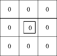
Fig.2 (a)                              Fig.2 (b)

I ( x - 1, y - 1)	I ( x - 1, y )	I ( x - 1, y + 1)
I ( x , y - 1)	I ( x , y )	I ( x , y + 1)
I ( x + 1, y - 1)	I ( x + 1, y )	I ( x + 1, y + 1)

Fig.1. Pixel I ( x , y ) of an image I

We define normalized self correlation function (NSCF) as:

A ( x , y ) =

∑∑ ( f ( x , y ) f ( x + k , y + l )) + ε k =- 1 l =- 1

k ≠ 0 l ≠ 0

8. f ( x , y )² + ε

such that 0 ≤ A ( x , y ) ≤ 1 and ε is a very small constant, i.e. ε 0.

After applying A ( x , y ) to whole image I , every pixel I ( x , y ) is replaced with I A ( x , y ) I . For applying A ( x , y ) to boundary pixels, the image has to be suitably padded.

NSCF will capture the variation in intensities around pixel   I ( x , y ) in a predefined neighborhood. If

δ [ I ( x , y )] denotes the intensity variation of pixels around pixel I ( x , y ) in neighborhood N , then I A ( x , y ) I → 1 if δ N [ I ( x , y )] → 0 i.e. I A ( x , y ) I .

maximum value for minimum variation in pixel intensities. Conversely, minimum value is assigned to I A ( x , y ) I for maximum variation in intensities or

• A.    Edge detection using NSCF

Edges in an image are replica of sharp discontinuities or local intensity variations. Processing an image having edges using NSCF, maps edge pixels to low intensities due to their very low correlation with neighboring pixels. For the same reasons, background pixels are mapped to high intensities as they are highly correlated to each other. Let image I ' is the result after replacing every pixel I ( x , y ) of image I by I A ( x , y ) I .

I —— I'

As explained above I ' has low intensity pixels at corresponding edge pixels in I and high intensity pixels at remaining coordinates. The edge map can be generated by taking negative of I ' .

Ie= λIn'                    (3)

where I is edge map of image I , I ^' is negative of I ^' and λ is a diagonal matrix of same size as I . λ can be used to adjust the intensity of pixels for display purpose.

• B.    Image segmentation using NSCF

Above we explain how NSCF can be used for edge detection or edge based segmentation of an image. Similarly, NCSF can be successfully exploited for region based segmentation. Fig.3 shows an image divided into two regions such that ‘region 1’ and ‘region 2’ have different sets of intensity variations i.e.

δ N [ R 1( x , y )] ≠ δ N [ R 2( x , y )].

Clearly, application of NSCF produces different outputs for each region and

IA(x, У)|R1 * A(X, У )|R2

This divides image into two set of intensities, producing a segmented image. For the region based segmentation, we can either use I or I depending upon suitability of results. Similarly, we can use A I or AI_n for further enhancement of results.

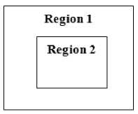
Fig.3. An image having two regions

• C.    Effect of neighborhood size

For simplification purpose we consider only odd size square neighborhood. We define variables a and b such that

(m-1) a = b =----- where m x m is neighborhood size.

For this general case (1) can be modified to:

A ( x , У ) =

k = a l = b

E E ⁽ f ⁽ x , y ) f ^{( x} + ^k , y + l )) + ⁸ k =- a l =- b k *— 0 l * 0

( m ² — 1). f ( x , y )² + 8

Considering larger neighborhood for calculating NSCF will take into effect the intensities of more pixels. This will help to take a better judgment about intensity variations around a particular pixel. This indirectly leads to better results as compared to smaller neighborhood size.

• D.    Effect of averaging

Fig.4(a) shows a 3 x 3 averaging filter which is used to replace a pixel I ( x , y ) with average value as calculated by the filter.

1/9	1/9	1/9
1/9	1/9	1/9
1/9	1/9	1/9

Fig.4(a). A 3 x 3 averaging filter

1	1	1
1	— 8	1
1	1	1

Fig.4(b). A 3 x 3 Laplace Filter

Averaging, indirectly increases the contribution of each pixel to the center pixel and hence increases the correlation between the pixels or reduces the variation of intensities in a predefined neighborhood. As expected, application of (5) after averaging will produce a brighter image which will produce a poor edge map.

• E.    Procedure for calculating NCSF of an image

The steps for calculating NSCF of an image I can be summarized as follows:

• 1.    Decide the neighborhood of odd size m x m .

• 2.    Calculate a and b using (2).

• 3.    Pad the image I to accommodate the boundary pixels in the neighborhood defined in step 1.

• 4.    At every pixel I ( x , y ) calculate A ( x , y ) using (5) and replace I ( x , y ) with A ( x , y ) . This will give image I .

• 5.    Using (3) find I^e or directly use I .

• III.    Relative Error Function

For quantitative description of algorithm, we propose relative error function (REF) which will also contrast the performance of two comparative algorithms. The motivation behind the approach is the assumption that a given algorithm applied to an image for an intended application will do so in the best possible manner leaving no scope for further modification by the second pass of the same algorithm. An image I can be mapped by a function F ( I ) to I^m .

I ^^-^. Im(6)

We define image I^m as

Im = I — | Im |

As the next step, we apply F ( I ) to I ^m to get I ⁿ .

Im   F( 1} > In(8)

F(I)  has already extracted all the relevant information in I m and subtraction ofIm from I will make I void of any information on which F(I)flourishes and therefore (8) should show maximum possible deviation from (6) i.e.

M - 1 N - 1

ZZ ( I m ( x , y ) - I n ( x , y ) ) should be maximum because x = 0 y = 0

smaller deviation implies the inability of the algorithm to target the relevant information in the very first pass. Next, we convert I^m and Iⁿ to respective binary images by calculating a suitable threshold such that both images have same pixels values for a particular range of intensities.

I n —— I B            (9)

I m —— I m           (10)

In this sense, I ^m and Iⁿ should have minimum possible deviation because a better algorithm in (8) will not spread the pixels to a greater range or otherwise deviation between I^m and Iⁿ can be used as quantitative measure of the algorithm. We tap this deviation in form of REF and define it as:

REF =

( M x N )

M - 1 N - 1

ZZ ( I m ( x , y ) © i b ( x , y )) x = 0 y = 0

where, © denotes ex-or operation and M x N is size of the image I . Clearly, REF measures the deviation between two images and should have minimum value for the betterment of the algorithm.

(a)                               (b)

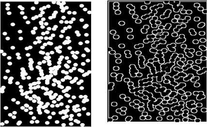
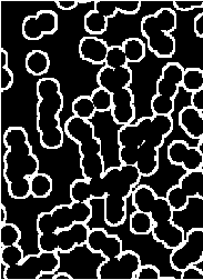
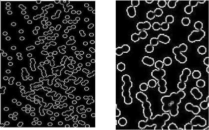
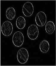
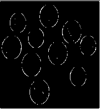
Fig.5. Results for image Bubbles. (a) Original image. (b) Result of Laplace filter. (c) Zoomed version of (b).(d) Result of NSCF. (e) Zoomed version of (d).

(c)

(d)                               (e)

b)

(f)

(g)

(h)

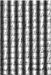
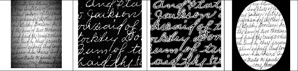
Fig.6. Results for image Shaded Text. (a) Original Image. (b) Result of Otsu’s method. (c) Result of 3 x 3 Laplace filter. (d) Result of 5 x 5 Laplace

filter. (e) Result of 3 x 3 NSCF. (f) Result of 5 _x 5 NSCF. (g) Result of 5 x 5 Laplace filter to image smoothed by 3 _x 3 averaging filter (h) Result of 5 x 5 NSCF to image smoothed by 3 x 3 averaging filter .

• IV.    Simulations and Results

NSCF is applied to various images for checking its correctness. We use objective assessment as well as quantitative assessment for the analysis of algorithm.

• A.    Objective assessment

For image Bubbles, the purpose is to extract the boundaries of objects. Comparison of fig.5(c) and fig. 5(e) shows that both Laplace filter and NSCF are able to extract the boundary of image but Laplace filter has distorted the shape of the boundary and has produced thick edges. It is also unable to extract the fine edges and has eliminated small objects. NSCF, on other hand, has produced undistorted image and is able to extract fine edges also. Overall, it has produced a natural boundary. The image Shaded text is used to check viability of NSCF for noisy case. Fig.6(b) shows the result of Otsu’s method which has clearly defeated its purpose. For the case of Laplace filter, fig.6(c) and fig.6(d) show that although method is able to threshold the image, the shaded strips are still appearing giving an unpleasant view. Further, the intensities of strips are enhancing with filter size, making the method unsuitable for noisy case. Fig.6(e) and fig.6(f) are for NSCF. It is evident that algorithm has naturally segmented the image by successfully combating the shaded strips and there is no evidence of shaded strips in the results. Moreover, the results of NSCF are improving with increased neighborhood size as already predicted. Fig.6(g) shows the result of Laplace filter after averaging

(a)                                       (b)                                        (c)                                        (d)

Fig.7. Results for image Spot shaded text (a) Original image. (b) Results of 5 x 5 Laplace filter. (c) Result of 5 x 5 NSCF. (d) Result of Otsu’s method.

(a)                                       (b)                                        (c)                                        (d)

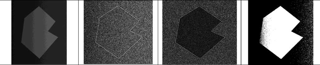
Fig.8. Results for image Noisy septagon (a) Original image. (b) Results of 5 x 5 Laplace filter. (c) Result of 5 _x 5 NSCF. (d) Result of Otsu’s method.

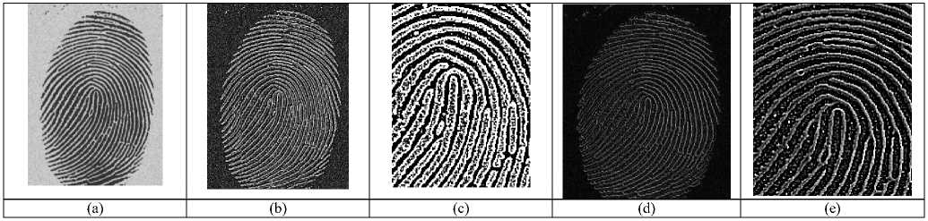
Fig.9. Results for image Thumb (a) Original image. (b) Results of 5 x 5 Laplace filter. (c) Zoomed version of (b). (d) Result of 5 x 5 NSCF. (e) Zoomed version of (d).

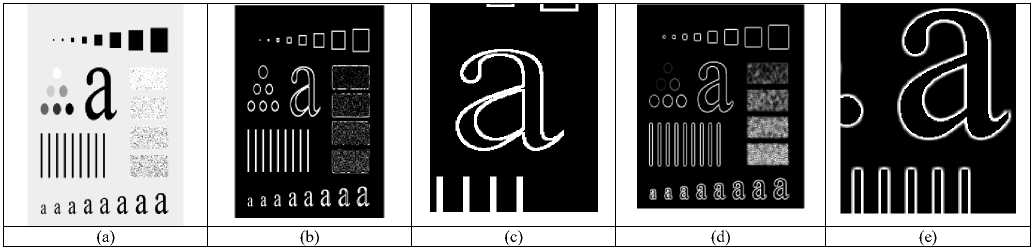
Fig.10. Results for image Pattern (a) Original image. (b) Results of 5 _x 5Laplace filter. (c) Zoomed version of (b). (d) Result of 5 _x 5 NSCF. (e) Zoomed version of (d).

the original image. Same results are shown for NSCF by fig.6(h). Laplace filter still has no effect on shaded strips while NSCF is producing even better result, a fact already proved in section II.

For image Spot shaded text in fig.7(a), the Laplace filter has produced ringing effect in background which is again an unnatural effect. Also, this effect will dominate with increased mask size. Otsu’s method has again failed for this case also and has produced a completely unnatural image. Coming to NSCF, it has again successfully segmented the image and has produced a uniform intensity image, leaving no clue of shaded spot in resultant image. The results can be further improved by either increasing the neighborhood size or averaging the original image before applying NSCF.

Image Noisy septagon in fig.8(a) has non uniform illumination with illumination increasing to right. The aim is to extract the septagon from background. Laplace filter failed completely for this case and is able to extract only the boundary of septagon which is obviously not our sole motive. Otsu’s method is able to threshold the image but with unnatural effect and clearly it is victim of non uniform intensity which is still appearing in the mapped image. NSCF has produced a fine image and has extracted septagon from background by assigning different intensities to foreground and background. Also, no sign of non uniform intensity exist in the results. In effect, non uniform intensity has no effect on the performance of NSCF.

For image Thumb in fig.9(a), Laplace filter has produced a noisy image with no clear extraction of details while NSCF has generated an image which is noiseless and from which fine details can be easily extracted. For image Pattern in fig 10(a), Laplace transform has produced thick edges with distorted boundary. NSCF for the same case has generated an image with perfect boundaries and thin edges.

• B.    Quantitative assessment

For quantitative assessment we use the relative error function (REF) defined in section III. We also calculate the execution time of the algorithm. Both quantities are calculated for each image with a neighborhood of 3 x 3 and no prior averaging. Results are depicted in table 1 and table.2.

Table 1. Calculation of REF for different images

Image	Algorithm
	NSCF	Laplace filter
Bubbles	.067	.192
Shaded text	.256	.470
Spot shaded text	.219	.459
Noisy septagon	.479	.502
Thumb	.249	.516
Pattern	.054	.178

From table.1. it can be concluded that the value of REF for every image is less in case of NSCF. As verified earlier in section III, a better algorithm should have minimum value of REF and hence quantitative assessment also proves that NSCF is way better than Laplace filter. Table 2 summarizes the execution time for both the algorithms. Execution time of NSCF differs from that of Laplace filter by a fraction of seconds which is negligible considering superior performance of NSCF over the later.

Table 2. Execution time (in sec.) for different images

Image	Algorithm
	NSCF	Laplace Filter
Bubbles	3.36	3.16
Shaded text	4.56	4.38
Spot shaded text	4.68	4.35
Noisy septagon	4.80	4.42
Thumb	7.30	6.84
Pattern	2.69	2.32

• V. Piecewise Image Segmentation

In this section, we propose a new algorithm that is useful for generating a controlled edge map of an image using a recursive approach. Traditional sharpening filter produces a relevant edge map in most of the cases but it has no provision for controlling the number of edges appearing in the edge map. Sometimes the requirement may be a partial edge map containing only the important edges like boundary pixels and void of all the minute edges. In such cases, traditional filters may not be a useful tools and we need to discover new methods. The proposed algorithm comes handy in such applications and presents a better alternative to the traditional filters. The algorithm operates recursively and can also produce complete edge map apart from partial edge map. In the remaining section develop the proposed algorithm and its methodology along with simulation results.

• A.    Methodology

Consider an image I of size M x N and an extension of the averaging filter f mentioned in fig.4 to size n x n , where n is an odd number. Using this filter we can calculate local mean at a pixel I ( x , y ) by the equation:

aa mL (x, У) = 55 I (x + k, У +1) f (k, l)    (12)

k=—a l=—a and for odd n, a = b = (n —1)/2. If we apply this operation at each pixel, then we get an image m having local mean as the pixels. Eq. (12) can be exploited to calculate the local variance at each pixel I(x, y) using:

aa

7 ( x , y ) =---- 5 5 [ I ( x + k , y + 1 ) — m_L ( x + k , y + 1 )]²

n X n k =— a l =— a

Similarly we can calculate the global mean as:

mG=(MN x 5 > y 5 >I (x •y)

and global variance as:

^G = (MXN) x 5.> y 5> (1 (x• y) - mG )2

Eq.(13) and (15) are basis for further development of the algorithm. Conceptually a pixel I ( x , y ) will belong to an edge if

-T ^ (7L (x• y) — 7G ) ^ T(16)

i.e local variance at the pixel lies within a particular range of global variance. This is an obvious condition because an edge pixel is identified by sudden change of intensity in its neighborhood and it will be reflected in its local variance which will be higher than global variance of the image.

Threshold T is used to check the output of the algorithm and it is also responsible for generating partial or complete edge map. In other words T induces a controlling nature in the algorithm. For different values of T a unique edge map is generated. Now, problem is to select the initial value and final value of the T.

As an initial step, we find the mean of 7 _L obtained using (13).

m =---~--- 5 5 7 (x• у)

• ⁷  ( M x N ) x =⁵ >  y ⁵ >  ^LV

Next, we find variance of G_L :

• <7 =-------- V V (ст, (x, y) — m )2

"  (M x N) x =5 > y 5n >  L

We use 7 as the initial value of T to start the iteration. Now, we find the maximum deviation between local variance and global variance i.e. G_L and 7 :

S = max{7 — 7 }

We use this deviation ( S ) as the final value of T in the iterations. The remaining of the algorithm will proceed as follows:

• 1)    With 7 as initial value of T and S as final value of T , start the iterations. Decide a predefined step size ( E ) and choose T + £ as the next threshold value. Repeat the following steps for each value of T till S is reached.

• 2)    If an pixel I ( x , y ) satisfies (16) then replace I ( x , y ) with output of Laplace filter ( w ) of predefined size (fig.4(b)) and centered at I ( x , y ) .

ab

I (x, У) =551 (x + k, У +1) w (k, l)

k =— a l =— b

• 3)    If an pixel I ( x , y ) fails (16) then

I (x, y) = 0

• 4)    Find global mean of the magnitude of image obtained after applying (2) and (3), say m ^' and also calculate

§ = mk — mk—1

• 5)    Find the value of T , say T_mш , for which § is maximum. This is the threshold value for which major changes in edge map will occur. All the

  other values of T including T and previous to T will produce a partial edge map. As we will move away from T in opposite direction, a lighter edge map will be obtained.

  The preferred value of T is

  
  

  T = T

  max

  
  

  —

  
  
  
  
  
  

  our preferred tool. The results of fig.12(c) were obtained by applying presented algorithm with threshold T which has successfully extracted the targeted region.

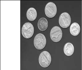
  For image Coins in fig.13, the aim is again to extract the boundaries of the objects. Laplace filter as usual (fig.13(b)) has produced a complete edge map. For this particular image, our algorithm with threshold T ax - 8 has extracted the boundaries of the coins but it is broken at some places. The threshold T would have max

  
  

This value will produce an edge map containing boundary pixels only and it can be exploited for boundary extraction of the object.

• B.    Objective assessment

The algorithm is tested on several images for verification of its performance. The results are obtained using filter of size 3 x 3. The results are summarized below:

For image Tower in fig.11, the Laplace filter has produced a complete edge map (fig.11(b) and results are fair in this sense but it’s not possible to extract boundary of the object using the same. The presented algorithm was applied with threshold Tm— 8 and it is successfully able to extract the boundary without concentrating on fine edges. If we further increase the threshold beyond T , we can replicate the results of Laplace filter.

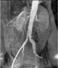
For image Kidney in fig.12, the complete edge map has lots of information but sometime the requirement may be produced an unbroken boundary but it had also generated more inner edges. Nevertheless, for such cases we can apply dilation to complete the boundary rather than increasing the threshold.

For image Moon in fig.14, the Laplace filter has again produced a complete edge map. The application of our algorithm with threshold Tm— 8 is able to extract the boundary but result (fig.14(c)) contains inner edges as well. Here, either we can further reduce the threshold value to Tm— 28 or we can apply erosion operation to get rid of minute inner edges.

For image Cameraman in fig.15, the expectations are same i.e. boundary extraction. The application of our algorithm has completely eliminated the background leaving only the boundary of main object in the image (fig.15(c)). If we try to recover the boundaries of background objects also by increasing the threshold value, then we may introduce unnecessary fine edges as in case of Laplace filter.

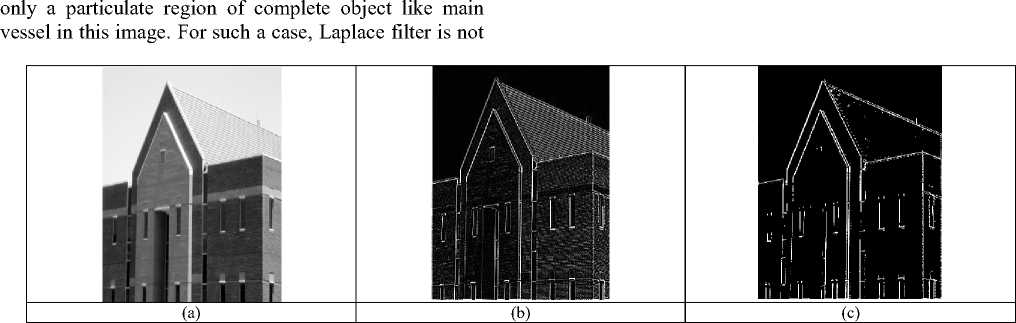
Fig.11. Results for image Tower. (a) Original image. (b) Result of 3 _x 3 Laplace filter. (c) Result of proposed algorithm with T _— 1 threshold.

(b)                                                   (c)

(a)

Fig.12. Results for image Kidney. (a) Original image. (b) Result of 3 x 3 Laplace filter. (c) Result of proposed algorithm with T threshold. max

(a)

(b)

(c)

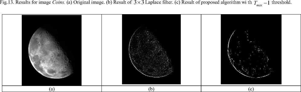
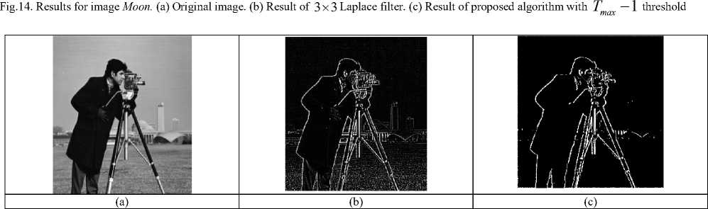
Fig.15. Results for image Cameraman. (a) Original image. (b) Result of 3 x 3 Laplace filter. (c) Result of proposed algorithm with T - 1 threshold.

• VI. Conclusion

This paper proposes two algorithms for image segmentation. Simulation results demonstrated that NSCF based algorithm performs well even in case of noisy or non-uniformly illuminated images. The REF also concludes that NSCF based algorithm is better than classic algorithm like Laplace filter even in qualitative sense. Moreover, this algorithm maintains its simplicity and has very less computational complexity. We also propose PIS as edge-based method which is successfully used in boundary extraction. In can also produce complete edge map like any other algorithm in this domain. However, we have not performed qualitative assessment of this algorithm.

• [1]    R.C. Gonzalez, R.E. Woods, and S.L. Eddins, Digital Image Processing . Upper Saddle River, NJ, USA: Prentice-Hall, 2004.

• [2]    A. Bovik, Handbook of Image and Video Processing . New York, NY, USA: Academic, 2000.

• [3]    H.K. Sawant and M. Deore, “A comprehensive review of image enhancement techniques,” Int. J. Comput. Technol. Electron. Eng . Vol. 1, pp. 39-44, Mar. 2010.

• [4]    J.C. Caicedo, A. Kapoor, and S.B. Kang, “Collaborative personalization of image enhancement,” in Proc. IEEE Conf. Comput. Vis. Pattern Recognit .,Jun. 2011, pp. 249256.

• [5]    Shuhang Wang, Jin Zheng, Hai-Miao Hu and Bo Li, “Naturalness Preserved Enhancement Algorithm for NonUniform Illumination Images,” IEEE trans. on Image Processing , Vol. 22, No. 9, 3538-2548, Sep 2013.

• [6]    N. R. Pal and S. K. Pal, “A review on image segmentation techniques,” Patt. Recognit ., vol. 26, no. 9, pp. 1277–1294, 1993.

• [7]    Anil K. Jain, Digital Image Processing .

• [8]    M. Kass, A. Witkin, and D. Terzopoulos, “Snakes: Active contour models,” Int. J. Comput. Vis ., vol. 1, no. 4, pp. 321–331, 1988.

• [9]    S. Osher and J. A. Sethian, “Fronts propagating with curvature dependent speed: Algorithms based on hamilton-jacobi formulations,” J. Comput. Phys ., vol. 79, no. 1, pp. 12–49, 1988.

• [10]    V. Caselles, F. Catt, T. Coll, and F. Dibos, “A geometric model foractive contours in image processing,” Numer. Math ., vol. 66, no. 1, pp.1–31, 1993.

• [11]    V. Caselles, R. Kimmel, and G. Sapiro, “Geodesic active contours,” Int. J. Comput. Vis ., vol. 22, no. 1, pp. 61–79, 1997.

• [12]    R. Malladi, J. Sethian, and B. Vemuri, “Shape modeling with front propagation: A level set approach,” IEEE Trans. Patt. Anal. Mach. Intell ., vol. 17, no. 2, pp. 158–175, Feb. 1995.

• [13]    X. Yang, X. Gao, J. Li, and B. Han, “A shape-initialized and intensity adaptive level set method for auroral oval segmentation,” Inf. Sci ., vol.277, pp. 794–807, 2014.

• [14]    X. Yang, X. Gao, D. Tao, and X. Li, “Improving level set method for fast auroral oval segmentation,” IEEE Trans. Image Process ., vol. 23, no. 7, pp. 2854–2865, 2014.

• [15]    X.Yang, X.Gao ,D.Tao, X.Li,and J.Li,“An efficient MRF embedded level set method for image segmentation,” IEEE Trans.Image Process .vol. 24, no. 1, pp. 9–21, 2015.

• [16]    C. Li, R. Huang, Z. Ding, J. Gatenby, D. N. Metaxas, and J. C. Gore,“A level set method for image segmentation in the presence of intensity inhomogeneities with application to mri,” IEEE Trans. Image Process ., vol. 20, no. 7, pp. 2007–2016, 2011.

• [17]    Y. Wang, L. Liu, H. Zhang, Z. Cao, and S. Lu, “Image segmentation using active contours with normally biased GVF external force,” IEEE Signal Process. Lett ., vol. 17, no. 10, pp. 875–878, 2010.

• [18]    S. Mukherjee and S. Acton, “Region based segmentation in presence of intensity inhomogeneity using legendre

  polynomials,” IEEE Signal Process. Lett ., vol. 22, no. 3, pp. 298–302, Mar. 2015.

• [19]    D. Mumford and J. Shah, “Optimal approximations by piecewise smooth functions and associated variational problems,” Commun. Pure Appl. Math ., vol. 42, no. 5, pp. 577–685, 1989.

• [20]    T. F. Chan and L. Vese, “Active contours without edges,” IEEE Trans.Image Process ., vol. 10, no. 2, pp. 266–277, 2001.

• [21]    Ashish Thakur and Radhey Shyam Anand, “A local statistics based region growing segmentation method for ultrasound medical images,” Int. J. of Signal Process. , Vol. 1, No. 2, pp 141-146, 2004.