The impact of road transport connectivity on economic growth of regions: econometric modeling

It is strategically important to strengthen the transport connectivity1 of territories (macro-regions, regions, core settlements, urban and rural areas, settlements within urban agglomerations, etc.), centers of economic growth, centers of scientific and technological development, enterprises and organizations that are links in the same value chains, participants in the same clusters, etc.) to ensure sustainable and balanced spatial development of Russia as the largest country in the world in terms of area. However, the range of positive effects that can be achieved by increasing transport connectivity of territories (improving the qualitative and quantitative characteristics of road and roadside infrastructure, means of transport, etc.), when examined in more detail, turns out to be wider and concerns not only the issues of effective organization of space and spatial development of territories.

For instance, strengthening transport connectivity in the economic sphere promotes the inflow of private investment, facilitates the entry of producers into new markets, reduces transport costs per unit of output by reducing economic and geographical distance, leads to the development of domestic tourism, facilitates the diffusion of innovations, increases the efficiency of the social division of labor, etc.2 (Isaev, 2015; Uskova, 2021; Yao, Liu, 2022; Zhu, Luo, 2022; Wang, Yang, 2023). Yu.A. Shcherbanin notes that “the importance of developed transportation infrastructure for the country’s economy is a kind of lemma, i.e. a proven statement...” (Shcherbanin, 2011).

Strengthening the transportation connectivity of territories in the social sphere increases the accessibility for the population of healthcare, education and other services guaranteed by the legislation of the country, raises the level and quality of life, contributes to the cultural integration of the country’s space (Khudyakova, 2015; Francisco, Helble, 2017; Rim, An, 2022).

From the point of view of public and national security, transport infrastructure provides manageability and connectivity of the country’s space, overcoming the periphery, economic, social, cultural isolation of territories (Gumenyuk, Gumenyuk, 2021; Taylor, D’Este, 2007), which is especially important for Russia in the conditions of external sanctions pressure, which aggravated the task of developing cooperation and integration ties within the country.

The variety of positive effects arising at the macro-, meso-, and microlevels when strengthening the transport connectivity of territories determines the development and implementation of special state programs and projects, for example, in Russia the national project “Safe Quality Roads”3, the Comprehensive Plan for Modernization and Expansion of Trunk Infrastructure4, the state program of the Russian Federation “Development of the Transport System”5. Moreover, one of the toplevel strategic planning documents – the Strategy for Spatial Development of the Russian Federation for the period up to 20256 – among the key tasks in the field of spatial development are identified overcoming infrastructure limitations of federal significance and increasing the availability and quality of trunk transport infrastructure, reducing the level of inter- and intra-regional differentiation by improving the transport accessibility of rural areas, etc. The Strategy for Spatial Development of the Russian Federation for the period up to 2025 is one of the key tasks in the field of spatial development.

However, despite the understanding of the critical importance of strengthening transport connectivity7, in particular road transport connectivity, by representatives of public authorities and the scientific community, the issues related to qualitative and quantitative assessments of its impact on the economic growth of Russian regions remain poorly studied and debated. In accordance with the abovementioned, the purpose of this paper is to assess the impact of road transport connectivity on the economic growth of Russian regions.

The research hypothesis is that the economic growth of each Russian region is influenced by the level of intraregional road transport connectivity of its own and other regions.

The purpose and hypothesis of the work required solving the following tasks: to substantiate and test the methodological approach to assessing the impact of road transport connectivity on the economic growth of Russian regions; to assess the impact of road transport connectivity of territories on the economic growth of Russian regions.

Theoretical and methodological foundations

Modern scientific literature can distinguish three main methodological approaches to assessing the impact of transport connectivity indicators on the territories’ economic growth of different hierarchical levels (countries, macro-regions, regions, municipalities, etc.). The first approach is associated with the use of new indices, indicators, indicators, matrices, etc. developed by the authors or already existing and publicly available; the second approach involves the use of traditional econometrics tools, mainly regression models; the third one implies application of methods and tools of spatial econometrics.

For example, we can include the study by E.S. Kuratova to the works that use the first approach to assess the impact of connectivity on various indicators of territories’ socio-economic development (Kuratova, 2014). It proposes the author’s formula for determining the weighted average cost of time required for a transportation user to reach a certain point of arrival (e.g., hospital, school, etc.) from any other departure points of the region; its testing was carried out on the example of municipal districts of the Komi Republic. The paper (Kudryavtsev, Rudneva, 2014) proposes a methodology based on a matrix for assessing the impact of transport infrastructure on the socioeconomic development of the region. In general, the key advantage of the first approach is the relative simplicity of calculations and interpretation of the results; the disadvantages are the lack of extensive testing and validation (this is mainly characteristic of new indicators), taking into account the impact of a relatively small number of indicators and the lack of opportunities for modeling and forecasting the impact, which is extremely important for the practice of public administration.

These shortcomings are mitigated by the use of econometric modeling tools (the second approach to impact assessment). By building regression models, researchers estimate, simulate and forecast the impact of various indicators of transport connectivity on the economic growth and development of one specific territory over a period of time (using temporal data; see, for example (Pyan’kova, Zako-lyukina, 2024)), several territories – within federal districts, individual clusters, etc.), at one point in time (when using spatial data; see, for example (Goridko, Roslyakova, 2014; Infrastructure of spatial..., 2020)), several territories within several points in time (when using panel data; see, for example (Kolchinskaya, 2015; Transport and energy ..., 2022)). It is worth noting that the construction of such models does not take into account the location of territories in the economic space relative to each other and spatial dependencies between them (the influence of some territories on others). Meanwhile, modern applied and fundamental theoretical works testify to the importance of taking into account the spatial factor. For instance, the basic and enduring, despite the active infrastructural development, laws of geography by W. Tobler say: “Everything is connected with everything, but close things are more connected than distant things”; “a phenomenon external to the area of interest (geographical) affects what happens inside it” (Tobler, 1970; Tobler, 2004).

This limitation is eliminated when using spatial econometrics tools, in particular, spatial autocorrelation indices and spatial regression models (the third approach to assessment). Unlike the tools and methods of economic research presented above, they allow assessing not only the impact of connectivity in the region on its economic growth, but also the impact of connectivity of its “neighbors”. This becomes possible by taking into account spatial lags – weighted average values of “neighbors” observations for each analyzed spatial unit (in our study – for each region). In this case, when choosing the boundary matrix as a weighting matrix, the regions that share a common border8 with it are the “neighbors” for the i-th region;

when choosing the inverse distance matrix, the “neighbors” are all other regions; when choosing the language matrix, the regions whose population speaks the same language, etc.

Among the Russian works that use this approach, the study by E.A. Kolomak (Kolomak, 2011) stands out, where econometric modeling with spatial lags is used to assess the impact of infrastructural capital on labor productivity and gross regional product, the idea of which is to expand the production function by including infrastructural capital and external effects of neighboring regions. At the same time, the author calculates Moran’s spatial autocorrelation index. According to calculations, transportation infrastructure, namely railroads and roads, was not an economic growth factor in Russia as a whole in Russian regions in 1999–2007. However, if we distinguish the western and eastern parts of the country, the situation changes: in the former, railroads turn out to be more productive and significant than in the latter, despite the widespread opinion about the limiting role of transportation infrastructure specifically in Siberia and the Far East. Moreover, infrastructure elements create externalities that affect the economic performance of neighboring territories; they are also stronger in the European part of the country (Kolomak, 2011).

A.G. Isaev’s work assesses the impact of transportation infrastructure – roads and railroads – on the economic dynamics of the RF constituent entities in 2000–2013. The multiple regression model built for this purpose, including the time lag of the dependent variable – gross regional product – allowed drawing extremely interesting conclusions. For example, the author revealed a positive relationship between the development of road transport networks and economic growth of Russian regions as a whole, and a negative relationship between the development of transport networks in a region and the economic growth of its neighboring regions (Isaev, 2015). In addition, the estimates obtained separately on the materials of the eastern territories of Russia did not reveal a positive contribution of transport infrastructure to regional growth (gross regional product), which is generally consistent with the results obtained earlier by E.A. Kolomak.

Spatial econometric tools are more actively used abroad to assess the transport connectivity of territories at different hierarchical levels (cities, regions, etc.). For instance, the paper (Shi et al., 2024) investigates the impact of transportation infrastructure on the economic development of PRC cities using Moran’s spatial autocorrelation and the construction of spatial regression models SAR, SEM, SDM. The results of the author’s calculations show that the growth of transportation by road and water transport, civil aviation significantly increases economic activity in cities, stimulating domestic trade, industrial production, etc. The expansion of the area and the rise in the operational length of urban roads and the length of expressways also stimulate economic activity. In contrast, the impact of road and water transport passenger traffic on economic activity was relatively insignificant, although the authors note that an efficient passenger transport system plays an undeniable role in facilitating labor mobility that supports sustainable urban development (Shi et al., 2024). The study (Karim et al., 2020) evaluated the impact of transportation infrastructure on economic growth of 34 provinces in Indonesia by constructing spatial regression models SLX, SAR, SEM, SDM, SDEM, SAC and mixed model SAC. The comparison of the models according to Akaike’ s information criteria and the significance of “rho” and “lambda” coefficients allowed choosing the best model among them, which turned out to be the mixed SAC model. Interpreting this model, the authors indicate that the development of provincial bus infrastructure has a positive and significant effect on economic growth in the neighborhoods (there is an indirect effect). Conversely, improving airport and road infrastructure in a province will not cause spillover effects in the form of transfer of production factors to neighboring provinces (Karim et al., 2020). Using a similar toolkit on the example of 41 cities located in the Yangtze River Delta (PRC), it was proved that the transport infrastructure of cities not only contributes to their own economic growth, but also has a positive spatial impact on the economic growth of neighboring cities in the sample (Wang et al., 2022).

In general, the review of scientific literature shows that the works of Russian authors devoted to assessing the impact of transport connectivity on the economic growth of Russian territories rarely take into account spatial dependencies in comparison with foreign works on similar topics. However, as noted by O.S. Balash, it is econometric models that take into account spatially distributed socioeconomic processes and detect the economic and social impact of neighboring regions that are extremely important for forecasting and management in the strategic planning of regions and cities (Balash, 2012).

Materials and methods

The information base of the research was the open data of Rosstat on the volume of gross regional product (in this study it acts as an aggregate indicator characterizing economic growth) and the level of development of road transport infrastructure in 2014–2022 in 83 constituent entities of the Russian Federation. Due to the lack of statistical data, information on the Donetsk People’s Republic, Lugansk People’s Republic, Zaporozhye Region, and Kherson Region was left out of the research. Table 1 gives the description of the variables used in the study.

The methodological approach to assessing the impact of transport connectivity on the economic development of Russian regions is imple- mented in three stages and is based on the use of spatial econometrics methods tested in the Russian and international scientific community.

At the first stage , the indicators selected for analysis are characterized using basic descriptive statistics (mean, maximum, minimum values, standard deviation), and the presence or absence of multicollinearity between exogenous variables is checked. At the same time, the variables that are found to be strongly correlated (correlation coefficient exceeds 0.7) are excluded from further analysis.

At the second stage , the global and local Moran’s spatial autocorrelation indices are calculated, and Moran’s scatter matrix is constructed for the endogenous variable and exogenous variables of interest⁹, which, within the framework of this study, will allow identifying the presence/ absence in the period 2014–2022 and the composition of clusters of regions similar in terms of GRP level, road density, number of passenger cars, etc., taking into account the measure of their spatial proximity. Such proximity of regions within the research framework is formalized on the basis of the weight matrix of inverse distances on highways between the administrative centers of the regions. Its choice among others is conditioned by the assumption of gradual “fading” of the intensity of interaction between territories as the distance between them increases. For comparison, the binary neighborhood matrix assumes that regions that do not have common borders have no interaction (Isaev, 2015).

In fact, the presence of clustering of regions confirms the relevance and necessity of taking into account spatial lags when assessing the impact of transport connectivity on the economic development of Russian regions.

Table 1. Variables used in the study

No.	Name of indicator, units of measurement	Designation	Data source or calculation method
Endogenous variable
1	Gross Regional Product (GRP), thousand rubles per 1 person	GRP	Calculated according to Rosstat data by dividing GRP converted to comparable prices in 2022 using the GRP physical volume index by the average annual number of population
Exogenous variables of interest
2	Density of public roads with paved surface, kilometers of tracks per 1,000 inhabitants	Road	Calculated according to Rosstat data by dividing the length of paved public roads by the average annual number of population
3	Share of rural settlements connected by paved roads to the public road network in the total number of rural settlements, percent	Rural_road	Rosstat (EMISS)
4	Number of passenger cars owned by citizens, units per 1,000 persons of the population	Car	Rosstat
5	Number of trucks in organizations, units per 1,000 persons of population	Truck	Calculated according to Rosstat data by dividing the number of trucks in organizations of all types of economic activity by the average annual number of population
6	Number of public buses, units per 100,000 inhabitants	Bus	Rosstat
7	Location of the constituent entity of the Russian Federation in the territory of the European or Asian North of Russia	Dummy	For subjects located in the territory of the European or Asian North of Russia, the variable is taken as “1”, outside it – “0”.
Exogenous control variables
8	Commissioning of residential buildings, square meters of total floor area of residential premises per 1,000 population	House	Rosstat
9	Volume of innovative goods, works, services, percentage of the total volume of shipped goods, works, services performed	Innov	Rosstat
Note: The European North of Russia includes the Arkhangelsk Region, with the Nenets Autonomous Area, the Vologda and Murmansk regions, the Komi and Karelia republics; the Asian North of Russia includes the Tyumen Region, including the Yamal-Nenets and Khanty-Mansi autonomous areas, the Krasnoyarsk Territory, the Republic of Sakha (Yakutia), the Chukotka Autonomous Area, the Magadan Region, and the Kamchatka Territory, all or most of the territory of which is located above the 60th parallel of the northern latitude. Indicator no. 3 for Saint Petersburg is assumed to be 100% due to the absence in the Rosstat database. When selecting the indicators included in the model, we took into account the availability of complete (without omissions) series of statistical data of Rosstat in the territorial (by regions) and temporal (by years) sections, which is the basis for the construction of balanced panels. The inclusion of the dummy variable is due to the objective need to take into account the specifics of the northern regions of the Russian Federation, characterized by the focal point of settlement, location of productive forces, infrastructure, the predominance of extractive industries in the economic structure, the complexity of natural and climatic conditions. Source: own compilation.

At the third stage, a multiple regression model is built on panel data, the use of which reduces the dependence between exogenous variables, reduces the standard errors of estimates, to a certain extent solves the problem of bias caused by unobserved heterogeneity of data, and has a number of other advantages over time and cross-sectional data. At the same time, certain assumptions / limitations due to the set of analyzed variables are taken into account when building the model. First, since the model contains exogenous variables that do not change over time (in particular, a dummy variable that takes the value of “1” and “0” throughout the analyzed period), a model with random effects was built. Second, the indicator of per capita GRP was included in the model in logarithmic form, since it is a cost indicator. As a result, the multiple regression model under construction is as follows:

In GRP_it = ft + ft x Road_it + ft x Rural_roadit +

+ ft x Car_it + ft x Truck_it + ft x Bus_it +

+ft x Dummy i + ft x House i _t + ft x Innov_it + щ + Ец, (1)

where GRP_it – GRP of the i -th region in year t , thousand rubles per 1 person;

Road_it – density of paved public roads in i -th region in year t , km of tracks per 1,000 population;

Rural_road – share of rural settlements in i-th _ it region in year t that are connected by paved roads to the public road network in the total number of rural settlements, %;

Car_it – number of passenger cars owned by citizens of i -th region in year t , units per 1 thousand people;

Truck_it – number of trucks in organizations of i -th region in year t , units per 1 thousand people;

Bus_it – number of public buses in i -th region in year t , units per 100 thousand people;

Dummy_i – dummy variable characterizing the location of i -th region (“on” or “outside” the territories of the European and Asian North of Russia);

House_it – commissioning of residential buildings in i -th region in year t , sq. m. of total floor area of residential premises per 1 thousand people;

Innov_it – volume of innovative goods, works, services in i -th region in year t , % of the total volume of shipped goods, works, services;

u_i – individual effect of i -th region (random variable);

• ε _it – random mistake;

• β – regression coefficients.

To test the hypothesis of the study, we constructed different model specifications most commonly used in similar works: without and with spatial lags, namely the spatial autocorrelation model SAR, which takes into account the lag in the dependent variable, the spatial error model SEM, which takes into account the mutual influence of unobserved variables, the spatial Durbin SDM model, which includes spatial lags of both the dependent and independent variables, the GSPRE model, which includes all kinds of spatial interaction10.

We made calculations according to the above methodological approach using Stata, Gretl, and Microsoft Office software products.

Research results

Descriptive statistics and assessment of correlation between the indicators selected for the study

Descriptive statistics of the variables used shows that the most uneven distribution among the regions of the Russian Federation is charac-

Table 2. Descriptive statistics of variables

Variable	Average value	Minimum	Maximum	Standard deviation
GRP	977.59	156.06	1262	1560.6
Road	13.8	0.5	47.0	7.6784
Rural_road	73.584	2.4	100.00	21.008
Car	301.06	38.437	576.22	70.998
Truck	4.9921	0.023959	23.883	2.6769
Bus	115.35	29.475	374.16	46.557
House	523.59	26.0	1970.0	261.06
Innov	5.3594	0.0	60.1	5.7791
Source: own compilation.

10 A detailed description and characteristics of the models are presented, for example, in (Gafarova, 2017).

Table 3. Correlation matrix

Variable l_GRP Road Rural_road Car Truck Bus Dummy House Innov l_GRP 1 -0.1143 -0.5595 0.1966 0.6002 -0.2494 0.6369 -0.0026 -0.0353 Road 1 -0.2834 -0.0920 0.3608 -0.1021 0.0836 -0.2092 -0.1779 Rural_road 1 0.0051 -0.5688 0.1501 -0.4258 0.1113 0.0152 Car 1 0.0285 -0.0138 0.1211 0.075 0.0472 Truck 1 -0.1998 0.4884 -0.0931 -0.0465 Bus 1 -0.1529 -0.018 0.0242 Dummy 1 -0.1968 -0.1711 House 1 0.1563 Innov 1 Note: hereinafter l_GRP is the natural logarithm of GRP. Source: own compilation. teristic of the indicators of per capita GRP (standard deviation is 1560.6, and the minimum and maximum values are 6.3 and 1.3 times less and 1.3 times more and less than the average value, respectively; Tab. 2) and the volume of commissioning of residential buildings (standard deviation is 261.06, the minimum and maximum values are 20 and 3.8 times less and more than the average value). In turn, the most uniform distribution is characteristic of the indicators of the number of trucks in organizations and the volume of innovative goods, works, and services.

We constructed a correlation matrix to identify the presence/absence of multicollinearity ( Tab. 3 ). According to the data presented in it, all exogenous variables are characterized by weak and moderate correlation dependence on each other (correlation coefficient less than 0.7), which allows them to be used further in this study.

Algebraic visualization of spatial autocorrelation

Table 4 presents the results of calculation of global Moran’s spatial autocorrelation indices characterizing the similarity of location to the studied endogenous variable and exogenous variables of interest in Russian regions. According to the 2022 results, positive spatial autocorrelation is recorded with respect to the indicators of per capita GRP, road density, the share of rural settlements connected to the public road network, the number of cars and trucks per 1 thousand people. It means that the regions characterized by higher values of any of the above indicators are usually neighboring with the regions that also have high values of the indicators. Regions with relatively low values of the indicators also neighbor predominantly with each other. Negative autocorrelation, which is much less frequent in scientific studies, was recorded with regard to the number of public buses per 100

Table 4. Global Moran’s spatial autocorrelation indices for endogenous variable and exogenous variables of interest

Variable	Год
	2014	2015	2016	2017	2018	2019	2020	2021	2022
GRP	0.046**	0.044**	0.042**	0.043**	0.047***	0.048***	0.050***	0.050***	0.047***
Road	0.052**	0.053**	0.054**	0.055**	0.056**	0.057**	0.057**	0.058***	0.059***
Rural_road	0.094***	0.099***	0.085***	0.091***	0.091***	0.090***	0.090***	0.088***	0.088***
Car	0.097***	0.094***	0.105***	0.058***	0.032	0.027	0.032*	0.037*	0.039*
Truck	0.124***	0.120***	0.093***	0.102***	0.099***	0.107***	0.086***	0.112***	0.096***
Bus	-0.018	-0.006	-0.009	-0.035	-0.019	-0.018	-0.033	-0.101***	-0.114***

Note: *** p-value < 0.01; ** p-value < 0.05; * p-value < 0.1. Source: own compilation.

thousand people. That is, regions characterized by a relatively high number of buses per 100,000 people are often adjacent to regions with a relatively low number of buses. This indicates a high degree of heterogeneity in the development of the public transportation system represented by buses in this study.

However, the most significant conclusion that follows from the results of calculating the global Moran’s indices, namely their statistical significance, is that spatial dependence should be taken into account when building a regression model of the impact of road transport connectivity on the economic growth of Russian regions.

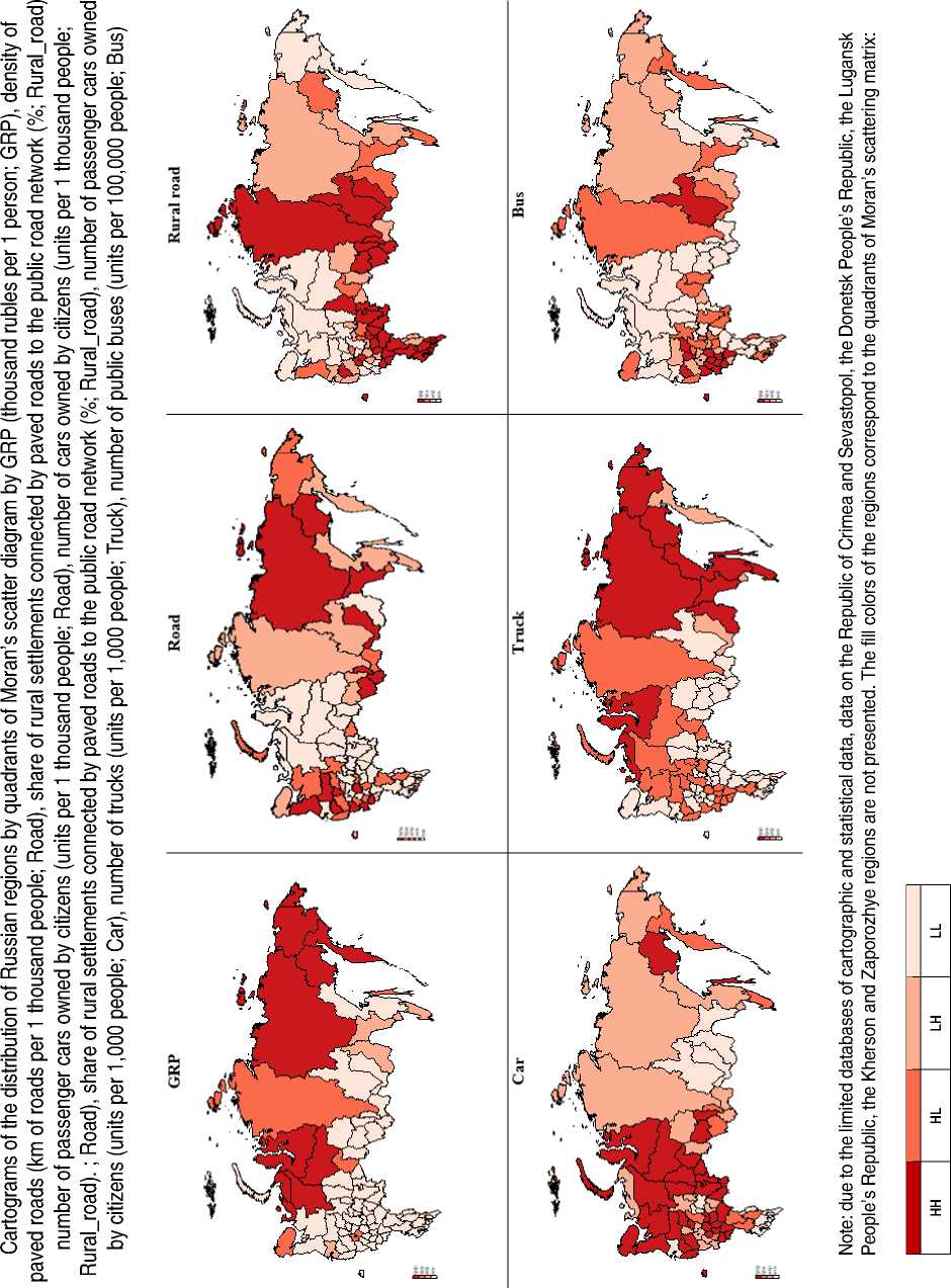
Cartographic visualization of spatial autocorrelation

The analysis of spatial autocorrelation with the help of Moran’s scatter diagram allowed distributing the studied Russian regions into four clusters (quadrants of the diagram) depending on the features of their spatial location and the level of the analyzed attributes. For instance, the regions in the HH (High-High) cluster have relatively high intrinsic values of the analyzed indicator and are surrounded by regions with relatively high values of the indicator. The regions of the LL (Low-Low) cluster, on the contrary, have relatively low eigenvalues of the analyzed indicator and are surrounded by regions with relatively low values of the indicator. Regions in the HL (High-Low) cluster have relatively high eigenvalues of the analyzed indicator, but are surrounded by regions with relatively low values of the indicator. The regions of the LH (Low-High) cluster, on the contrary, have relatively low eigenvalues of the indicator, but are surrounded by regions with relatively high values of the indicator. With a certain degree of conventionality, we can say that the regions of clusters HH and HL represent the centers / cores characterized by the highest values of the analyzed indicators, while the regions of clusters LL and LH are peripheral territories.

The Figure demonstrates the cartographic visualization of the regions’ distribution by endogenous variable and exogenous variables of interest. In general, it visually confirms once again the presence of positive spatial autocorrelation among the constituent entities of the Russian Federation, i.e. that the subjects are not located chaotically, but form territorial clusters.

It is interesting and quite expected that the cartograms coincide to a certain extent for the indicators of per capita GRP and the number of trucks in organizations, since in Russia the leaders in terms of GRP per capita are mainly northern regions, where the extractive and manufacturing industries have a significant share in the economic structure. It is truck transportation that ensures its uninterrupted functioning (supply of raw materials, materials, equipment, sales of finished products, transportation of semi-finished products between shops, etc.)11. At the same time, a significant part of the regions of the Northwestern (e.g., the Komi Republic, the Arkhangelsk, Murmansk, and Vologda regions) and Ural (the Tyumen Region, the Khanty-Mansi and Yamal-Nenets autonomous areas) federal districts are in the HH cluster in terms of the number of passenger cars per 1,000 people, and in terms of road density per 1,000 people, it is LL cluster. In our opinion, this confirms with a certain degree of conventionality the well-known thesis about the underdevelopment of road infrastructure in Russia’s northern regions.

Output of spatial multiple regression models results

Within the framework of the study, 5 model specifications for panel data with random effects were constructed (Tab. 5) . At the same time, one of the main issues is the choice of one best model among the presented models. First of all, it is worth noting that the results of Moran’s spatial autocorrelation analysis indicate that it is reasonable to take spatial effects into account in the model (accordingly, the model without taking spatial effects into account is excluded from further analysis).

To select the best model among SAR, SEM, SDM and GSPRE, the Akaike and Schwartz information criteria and the adjusted coefficient of determination were compared. This allowed identifying as the best model SDM, which is characterized by the lowest value of the Akaike (-2,086) and Schwartz (-1,994) coefficients, the highest value of the coefficient of determination (0.466). Table 6 presents more detailed descriptive statistics of the SDM model, including spatial lags and spatial effects.

Table 5. Model estimation results for panel data with random effects with and without spatial lags

Indicator	Model specification
	No spatial effects	With spatial effects
		SAR	SEM	SDM	GSPRE
Regression estimates
Road	0.012***	-0.000	-0.003	-0.005**	-0.005**
Rural_road	-0.001	-0.000	-0.000	-0.000	0.000
Car	0.001***	0.000***	0.000**	0.000	0.000*
Truck	-0.005***	-0.006***	-0.007***	-0.007***	-0.007***
Bus	-0.000**	0.000	0.000	0.000*	0.000
Dummy	0.532***	1.134***	1.259***	0.963***	1.101***
House	0.000	0.000	-0.000	-0.000	-0.000
Innov	-0.001	0.000	0.001*	0.001**	0.001
Constant	6.035***	0.980***	6.294***	3.760***	6.298***
Spatial autocorrelation coefficients
Spatial
rho		0.822***		0.463***
lambda			0.895***		1.097***
phi					1.691***
Variance
lgt_theta		-3.567***		-3.585***
sigma2_e		0.002***	0.002***	0.002***
ln_phi			5.186***
sigma_mu					0.497***
sigma_e					0.041***
Akaike Information Criteria (AIC) and Schwartz Information Criteria (BIC)
AIC	1651	-2033	-2013	-2086	-2017
BIC	1689	-1977	-1957	-1994	-1957
Adjusted coefficient of determination
R-squared		0.437	0.405	0.466	0.404
Note: *** p-value < 0.01; ** p-value < 0.05; * p-value < 0.1. The dependent variable is l_GRP. The significance of inclusion of the dummy variable was confirmed by the Wald test. The number of observations is 765 units. Algebraic form of the SDM model: In GRP = 3.760 — 0.005 x Road — 0.000 x Ruralroad + 0.000 x Car — 0.007 x Truck + 0.000 x Bus + 0.963 x Dummy — — 0.000 x House + 0.001 x Innov; under the model under consideration, all other things being equal, the GRP of the regions comprising the European and Asian North of Russia (Dummy = 1) is almost 2.6 times higher than the GRP of other regions (Dummy = 0). Source: own compilation.

Table 6. Regression estimates, spatial lags and spatial effects model for panel data with random effects with SDM spatial lags

Variable	Regression coefficients ( β )	Spatial lags in exogenous variables (Wx)	Direct effects (LR_Direct)	Indirect effects (LR_Indirect)	Total effects (LR_Total)
Road	-0.005**	0.045***	-0.004*	0.080***	0,076***
Rural_road	-0.000	-0.017***	-0.001	-0.033***	-0.034**
Car	0.000	0.001*	0.000	0.001*	0.001**
Truck	-0.007***	0,005	-0.007***	0.004	-0.003
Bus	0.000*	-0.000	0.000*	-0.000	-0.000
Dummy	0.963***	1.583	1.014***	3.772	4.787**
House	-0.000	0.000**	-0.000	0.000**	0.000***
Innov	0.001**	-0.004	0.001*	-0.006	-0.005
Note: *** p-value < 0.01; ** p-value < 0.05; * p-value < 0.1. Source: own compilation.

Based on the results of the calculations, we can draw the following key conclusions regarding the SDM model.

• 1.    The spatial autocorrelation coefficient rho¹² in the model under consideration is statistically important at the 1% significance level (see Tab. 5). This means that there are global spillover effects, reflecting the influence on the per capita GRP of each particular region not only of its immediate neighbors, but also of the neighbors of the second, third, etc. order. The positive sign of the coefficient indicates that the growth/decrease of GRP in one region results in the growth/decrease of GRP in neighboring regions¹³ (Demidova, Timofeeva, 2021), assuming the same influence of neighboring regions on each region, i.e. the constancy of the rho coefficient.

• 2.    The coefficient at spatial lags theta¹⁴ is statistically significant and negative. This allows saying that as the values of exogenous variables in neighboring regions increase, the opposite changes of the endogenous variable occur in the region

• 3.    Since in the spatial model among the explanatory factors, there are spatial lags of independent variables, it is necessary to interpret not the coefficient estimates, but the estimates of spatial effects for the factors under consideration (Demidova, Timofeeva, 2021). Table 6 presents the effects calculated on average for all 83 Russia’s regions analyzed. According to these data, in particular the average overall effect, the change in gross regional product in each i-th region is statistically significantly affected by the change in all regions of the indicators 1) road density, 2) the share of rural settlements connected by paved roads to the public road network, 3) the number of passenger cars, 4) the location of the RF constituent entities in the European or Asian North of Russia, 5) the per capita volume of commissioning of residential buildings, with the second one having a negative effect, and the second one having a negative effect.

under consideration (assuming the same influence of neighboring regions on each region, i.e. the constancy of theta coefficient).

In general, the SDM model confirmed the statistically significant impact of road density (lag 0.045; see Tab. 6), the number of passenger cars (lag 0.001) per 1,000 population, and the share of rural settlements connected by paved roads to the public road network (lag -0.017) in neighboring subjects on each region. The positive impact of road density and the number of motor vehicles of citizens looks quite natural: with their increase, the population and businesses get additional opportunities to make more business, tourist and other trips, including to neighboring regions15. If we take into account that the main GRP volume is created mainly in cities and urban agglomerations, in urban-type mining/processing settlements, the negative impact of increasing the connectivity of rural areas also looks natural with a certain degree of convention. However, in our opinion, this should not become a determining factor for federal and regional government authorities when making decisions on the development of the country’s transport infrastructure; it is necessary to take into account the overall social significance of increasing the connectivity of rural areas in the country’s space.

In addition, the analysis of direct spatial effects allows concluding that the greatest positive and statistically significant impact on the volume of per capita GRP of the i-th region has the factor concerning the region’s location in the European or Asian North of Russia. This is generally explained by the resource specialization of the economy of the northern territories, which helps to form a significant GRP volume, and their relatively low population density. In turn, as a result of the analysis of indirect spatial effects, we can conclude that the greatest positive and statistically significant impact on the volume of per capita GRP of the i-th region is produces by the density of roads in other Russia’s regions, due to the fact that roads are the main type of infrastructure used for the movement of the population, representing the key final consumer in the economic system, demanding a huge number of goods, works and services.

In general, most indicators of road transport connectivity are characterized by a complex role in increasing the GRP level of Russian regions, since the signs of direct and indirect effects for the same indicators are different in most cases.

Conclusions

The study assesses the impact of road transport connectivity on the economic growth of Russian regions. For this purpose, we propose a methodological approach based on the spatial econometrics toolkit. Its application allowed obtaining the following key results.

First, by calculating Moran’s spatial autocorrelation coefficients, we found that there is a positive spatial autocorrelation among the RF constituent entities in terms of per capita GRP and most indicators of motor transport connectivity (road density, the share of rural settlements connected to the public road network, the number of cars and trucks per 1,000 people). As a rule, regions characterized by higher values of any of these indicators are adjacent to regions that also have high values of the indicators. Regions with relatively low values of indicators also neighbor predominantly with each other. It means tat the subjects are not located chaotically, but form territorial clusters, directly visualized on cartograms. At the same time, the statistical significance of global Moran’s indices for the variables used in the study indicated the need to take into account spatial dependence when building a regression model of the impact of road transport connectivity on regional economic growth.

Second, the construction and then comparison of several regression models with and without spatial lags allowed establishing that the best model is the SDM model, which takes into account lags for endogenous and all exogenous variables. In the course of its interpretation, we revealed that spillover effects take place in the Russian regions in terms of per capita gross regional product: the GRP level of each region is positively affected by the level of GRP of its neighbors of the first, second, third, etc. order. At the same time, the change in gross regional product in each i-th region is statistically significantly influenced by the change in all Russian regions in such indicators of motor transport connectivity as the density of roads per 1,000 people, the share of rural settlements connected by paved roads to the public road network, the number of passenger cars per 1,000 people. Thus, the hypothesis that the impact of road transport connectivity on the economic growth of Russian regions is due to the spatial location of the regions can be considered partially confirmed.

The theoretical significance of the study consists in the substantiation of the dependence of the economic growth of each constituent entity of Russia on the level of intra-regional transport connectivity not only of its own, but also of other regions (in the period 2014–2022). The practical significance lies in the possibility of using the results by the government authorities of the federal and regional levels in improving the policy in the sphere of socio-economic and spatial development of territories.

However, realizing that the results of the conducted research do not provide a comprehensive and complete answer regarding the established in Russia patterns of influence of transport connectivity on economic growth, it is necessary to highlight the prospects for further work:

• –    assessment of the impact of road transport connectivity on economic growth taking into account the different sensitivity of each region to the impact of other regions of the Russian Federation, i.e. taking into account the assumption of the non-constancy of the spatial coefficients rho and theta;

• –    construction of spatial regression models of GRP dependence on indicators of motor transport connectivity for different groups of regions according to their attribution to the HH, HL, LH, LL Moran’s clusters;

• –    modeling the impact on the economic growth of the constituent entities of the Russian Federation of railway, water, aviation and, in general, integrated transport connectivity (for all modes of transport), taking into account the gaps in statistical data;

  – analysis of the problems that can offset the positive impact of road transport connectivity on the economic growth of Russian regions: inconsistency of planned guidelines for transport and economic development, weak involvement of transport infrastructure in the economic processes of the region, etc. (Roslyakova, 2021).