The influence of economic growth on the financial sector by example of Portugal

The financial system comprises all financial markets, instruments and institutions. Today I would like to address the issue of whether the design of the economic system matters for the growth of the financial sector. My view is that the answer to this question is yes. According to cross-country comparisons, individual country studies as well as industry and firm level analyses, a positive link exists between the sophistication of the economic growth and the financial sector. While some gaps remain, I would say that the financial system is vitally linked to economic performance. Nevertheless, economists still hold conflicting views regarding the underlying mechanisms that explain the positive relation between the degree of of the economic growth and financial sector development.

Some economists just reject the idea that the finance-growth relationship is vital. For instance, Robert Lucas asserted in 1988 that economists badly overstress the role of financial factors in economic growth. Moreover, Joan Robertson declared in 1952 that " where enterprise leads, finance follows" . According to this view, economic development creates demands for particular types of financial arrangements, and the financial system responds automatically to these demands.

Other economists strongly believe in the importance of the economic growth for the financial sector. They address the issue of what the optimal economic system should look like. Overall, the notion seems to develop that the optimal financial system, in combination with a well-developed legal system, should incorporate elements of both direct, market and indirect, bank-based finance. A well-developed financial system should improve the efficiency of financing decisions and thereby favoring a better allocation of resources.

LITERATURE REVIEW

Most quantitative literature on international reserve holdings is based on theories developed in the 1960s, when the world adhered to the Bretton Woods System and the global capital flows were relatively small. The framework of analysis on reserve adequacy and optimality could be classified by the methodologies used into two categories: ratios as tools of analysis and regression analysis. The following gives a chronological retrospect of previous study.

Ratio AnalysisReserve to import ratio

The most widely used ratio method was the ratio of reserve to import first generalized by Triffin (1947, 1960). It is argued that the demand for reserves should move in line with the trend in international trade since receipts and payments were observed to be volatile. He concludes that major countries should maintain a constant reserve to import ratio ranging from 20 percent as a minimum to 40 percent maximally.

However, this method was born with almost equal number of critics and advocators. Machlup (1966) discredits the theoretical basis for the assumed rigid reserve-import ratio as it lacks of evidence and theory on why such ratio should remain constant across countries or through time. As his defense, three other ratios, including reserve to largest annual reserve losses, reserve to domestic money and quasi money, reserve to liabilities of central banks, were used to explain the behaviors of 14 industrial countries from 1949 to 1965. He stated that “on purely economic grounds, reserves are held only for the purpose of being eventually used.” However, this ex parte assumption also neglects a precautionary nature of reserves, especially under fixed exchange rate regime. Similarly, Olivera (1969) theoretically argues that precautionary demand for reserves should reflect variance of changes in annual imports, implying that a constant reserve-import ratio leads to a significant overestimation of present and future demands. 6

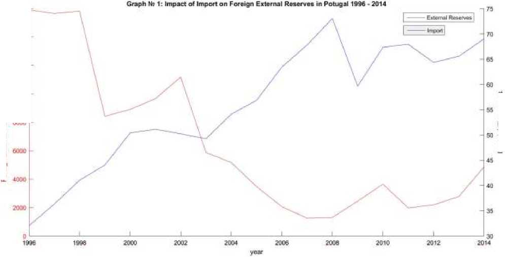
The IMF started to measure the adequacy of reserves in the 1950s by the ratio of reserve to import. European Central Bank (2006) regards four months’ import coverage as the “rule of thumb”. Since the major function of foreign exchange reserves is protecting a country from the uncertainty of international trade, the ratio of reserve to import has almost been included in all analysis on this subject.

Impact of Import on Foreign External Reserves in Portugal from 1996 to 2014 is depicted on the graph № 1

1000€ p

14000 -

13000 -

600€

Foro«gn External Reserve» hliion auras

soma suoiihi роки]

Reserve to domestic money supply

Because enough stockpiles of international reserves would substantially improve the credibility of a country’s currency, the ratio of reserve to domestic money indicates the potential of capital flight from domestic currency. Machlup (1966) was the first one who managed to use this ratio, although he finally obtained a contradictory conclusion that the demand for reserves is independent of any identifiable variable. The procedure of the functioning of reserve holding is nevertheless sound while ratios act unstable through time. This evidence is proved by Frenkel (1971), who performed a regression equation on 55 countries, 4

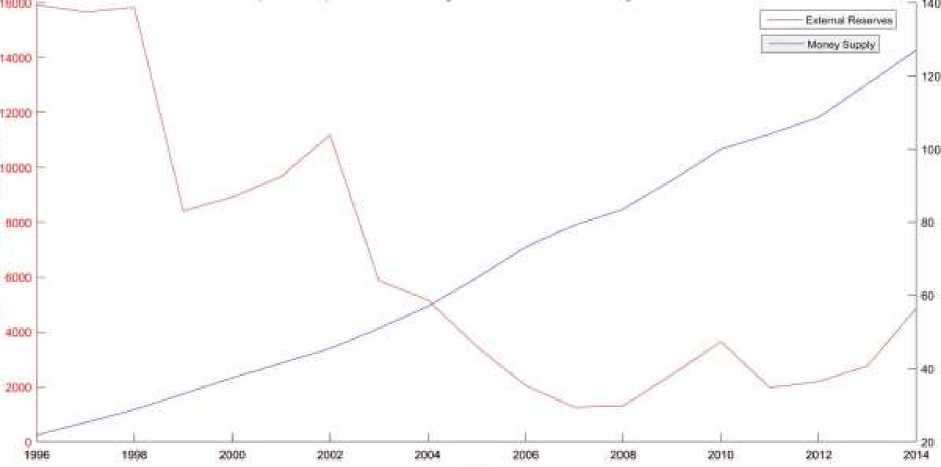
and the coefficient of domestic money supply was statistically significant, especially for less developed countries. Furthermore, Frenkel and Johnson (1976) expatiate that international reserves will increase if the demand for money exceed supply and vice versa. In that sense, international reserves are a residual. Based on this view, Frenkel (1978) suggests combine the demand for international reserves theory and the monetary approach to the balance of payments, followed by an attempted analysis by Lau (1980). Interestingly, Edwards (1984) empirically explores the relationship between reserve flows and domestic credit creation by using 23 fixed exchange rate developing countries and concludes that domestic credit cannot be considered completely exogenous but partial evidence.

Impact of Money Supply (M1) on Foreign External Reserves in Portugal from 1996 to 2014 is depicted on the graph № 2

Graph Ite 2: Impact of Mt on Foreion External Reserves tn Potuoal 1996 -2014

Fensign Esiurnal Reserves billion euros

Money Supply. |10Q я 2005)

Reserve to debt ratio

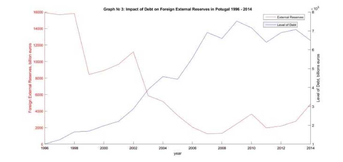
Brown (1964) gives an analysis of the reserve to net external balance ratio on the ground that reserves function as a cushion against future balance of payments deficits. It is assumed that this ratio reflects an economy’s financial ability to serve its existence.

External debts, especially in times of a sudden stop in short-term external debt flows. Greenspan and Guidotti (1990) suggest that developing countries, with limited access to international capital market, should at least cover all their debts.

Impact of External Debt on Foreign External Reserves in Portugal from 1996 to 2014 is depicted on the graph № 3

AN OVERVIEW OF MACROECONOMIC SITUATION IN THE COUNTRY

Background

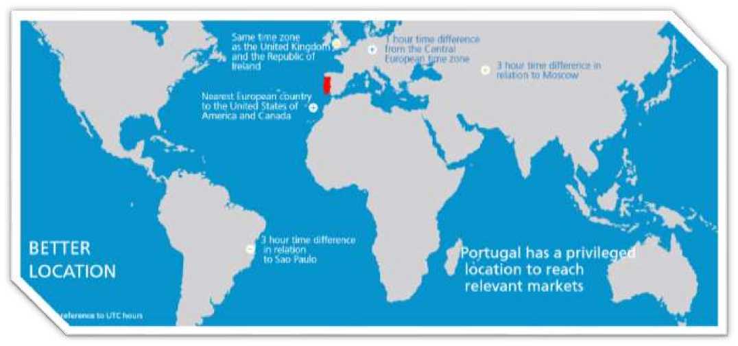
Mainland Portugal is geographically located in Europe’s West Coast, on the Iberian Peninsula. It is bordered by Spain to the North and East and by the Atlantic Ocean to the West and South, therefore being in a geo strategic location between Europe, America and Africa.

In addition to the mainland, Portugal’s territory also includes the Autonomous Regions of the Azores and Madeira, two archipelagos located in the Atlantic Ocean.

Portuguese borders have remained unchanged since the XIII Century, making Portugal one of the oldest countries in the world, with nearly 900 years of history that clearly demonstrates its strong identity and internal cohesion.

Population

Portugal’s population is estimated at 10.3 million, of which 50% are economically active. The demographic concentration is higher near the coastal areas, with Lisbon (the capital city) and Porto showing the highest population density.

Politics

The Republic of Portugal is a Parliamentary democracy, based on the respect and the effective guarantees for fundamental rights and freedoms and the separation and interdependence of powers. Under the Portuguese Constitution, sovereign powers are vested in the President of the Republic, the Assembly of the Republic, the Government and the Courts.

The current President of the Republic is Marcelo Rebelo de Sousa, who was elected in January 2016.

Legislative power lies with the Parliament (Assembly of the Republic) represented by 230 members which are elected by popular vote to serve a four-year term.

Executive power lies with the Government, headed by the Prime Minister, the Ministers and the Secretaries of State. The current Prime-Minister is António Costa, leader of the socialist party, who took office in November 2015.

Table 1. Portugal Economics Data Summary. Source: INE (National Statistics Office), Banco de Portugal

Area:	92 212 .0 sq km
Population (thousands):	10 337 (2015)
Working population (thousands):	(thousands): 5 195 (2015)
Population density (inhabit./sq km):	112.6 (2015)
Official designation:	Republic of Portugal

Capital:	Lisbon (2.1 million inhabit.– metropolitan area)
District Capitals:	Aveiro, Beja, Braga, Bragança, Castelo Branco, Coimbra, Évora, Faro, Funchal (in Madeira), Guarda, Leiria, Ponta Delgada (in the Azores), Portalegre, Porto, Santarém, Setúbal, Viana do Castelo, Vila Real and Viseu.
Main religion:	Roman Catholic
Language:	Portuguese
Currency:	EUR = 1.1212 USD (average rate in August 2016)

Picture 1. Portugal Geography. Source: INE (National Statistics Office), Banco de Portugal

Infrastructures

As a member of EU Portugal is undoubtedly a country with a highly developed infrastructure. It is comprised of:

Road Infrastructures: Portugal has a developed road network, comprised of motorways (AE), main roads (IP)

Rail Network: The rail network comprises 2 544 km providing North-South connection down the coastline and East-West across the country.

Airports: There are 15 airports. On the mainland the three major international airports are located in the coastal cities of Lisbon, Porto and Faro.

Economy

Economic structure

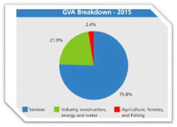
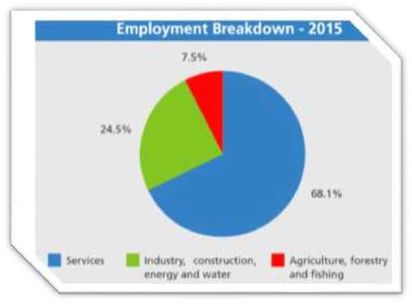
Following the trend of its European partners, over the last decades one of the most important characteristics of the structure of the Portuguese economy is the increase in the services sector that contributed, in 2015, with 75.8% of GVA and employed 68.1% of the population. Agriculture, forestry and fishing generated only 2.4% of GVA and 7.5% of employment while industry, construction, energy and water represented 21.9% of GVA and 24.5% of employment.

Picture 2. GVA Breakdown – 2015. Source: INE (National Statistics Office) Note: GVA - Gross Value-added

Picture 3. Employment Breakdown – 2015. Source: INE (National Statistics Office)

Current economic situation and outlook

In May 2014, the Government announced the end of the Economic and Financial Assistance Programme - PAEF (agreed with the EU and the IMF in May 2011), without resorting to additional external financial assistance thus gaining access to international debt markets.

After three years of the Programme, the Portuguese economy has made significant progresses in the correction of a number of macroeconomic imbalances, having implemented measures of a structural character in several areas.

In 2015, according to the INE (National Statistics Office), the Portuguese economy registered an increase of 1.5% in volume, year on year (after +0.9% in 2014 and -1.1% in 2013). This recovery was due to the positive performance of domestic demand (+2.5% in relation to 2014), reflected in the increase of private consumption (+2.6%) and an increase in public consumption (+0.6% in relation to the previous year, after various years of successive falls). Also the gross fixed capital formation increased in 2015 (+4.1%).

According to the same source, the increase of real export growth in goods and services was 5.2% during the last year (with the goods sector increasing 5.9% and services 3.1%), while imports increased 7.6%. The combined current and capital account balance in 2015 was positive, achieving 1.7% of GDP.

In the 2nd quarter 2016, according to INE, GDP registered an increase of 0.9% in volume, year on year.

Table 2. Portugal Economic Indicators 2012-2016. Sources: INE - National Statistics Office, Banco de Portugal, European Commission, Eurostat

Notes: (a) Forecast: Banco de Portugal (June 2016), European Commission (European Economic Forecast - Spring 2016)

	Economic Indicators	2012	2013	2014	2015	2016
GDP	Million EUR	168 398	170 269	173 446	179 369	184 477
	Real change	-4.0	-1.1	0.9	1.5	1.3
	Million USD	216 358	226 135	230 423	199 010	208 459
Per capita (PPS)	EU = 100	79	80	80	79	79
Private consumption	Million EUR	111 610	111 144	114 360	118 184	121 151
	Real change	-5.5	-1.2	2.2	2.6	2.1
Public consumption	Million EUR	31 177	32 501	32 165	32 534	33 332
	Real change	-3.3	-2.0	-0.5	0.6	1.1
Investment/GFCF	Million EUR	26 672	25 122	25 772	26 974	27 583
	% of GDP	15.8	14.8	14.9	15.0	15.0
	Real change	-16.6	-5.1	2.8	4,1	0.1
GFCF (excl. construction)	% of GDP	6.9	7.0	7.4	7.5	n.a.
	Real change	-11.8	4.1	9.3	4.0	n.a.
Population	‘000 inhabitants	10 515	10 457	10 401	10 358	10 299
Employment	‘000 individuals	4 581	4 450	4 513	4 576	4 616
Unemployment	‘000 individuals	836	855	726	647	595
Rate of economic activity	% of total population > 15 years old	60.2	59.3	58.8	58.6	n.a.
Unemployment rate Portugal	% of active population	15.5	16.2	13.9	12.4	11.6
Overall balance - General Government	% of GDP	-5.7	-4.8	-7.2	-4.4	-2.7
Public Debt	% of GDP	126.2	129.0	130.2	129.0	126.0
Current Account Balance	Billion EUR	-3.0	2.6	0.1	0.8	0.6
	% of GDP	-1.8	1.5	0.1	0.4	0.3

HCPI – Portugal	Annual change – average	2.8	0.4	-0.2	0.5	0.7
HCPI – Euro Area	Annual change – average	2.5	1.3	0.4	0.0	0,2

International trade

According to data released by the Banco de Portugal, in the last five years exports and imports of goods and services registered annual average growth rates of 4.9% and 1.2%, respectively. The trade balance of goods and services was positive between 2012 and the 1st half 2016, inverting the negative tendency registered in the past.

Table 3. Portugal International Trade (Goods and Services) 2011-2016. Source: a) Banco de Portugal (Trade in Goods and Services); b) INE -National Statistics Office (Trade in Goods);

Portugal’s International Trade              2011 Trade in goods and services (a)			2012	2013	2014	2015	Var. % 2015/2011c	2016 Jan/Jun	Var. % 2016/2015
Exports (fob)	Million EUR	42 828	45 213	47 303	48 054	49 826	3.9	24 811	-1.4
Imports (fob)	Million EUR	59 551	56 374	57 013	59 032	60 310	0.4	29 816	-1.4
Balance (fob)	Million EUR	-16 723	-11 161	-9 710	-10 978	-10485	--	-5 005	--
	% of GDPe	-7.9	-5.0	-4.0	-4.6	-4.3	--	-4.2	--

With regards to exports and imports of goods, in the first half 2016 there was a reduction of 1.4% in both over the same period, according to date from INE (National Statistics Office), corresponding to a coverage ratio of 83.2%. The trade balance of goods continues to show a deficit in the first half 2016, verifying, however, a reduction over the same period.

Table 4. Portugal International Trade (Goods) 2011-2016. Source: INE – National Statistics Office

Portugal’s International Trade		2011	2012	2013	2014	2015	Var. % 2015/2011c	2016 Jan/Jun	Var. % 2016/2015
Trade in goods(a)
Exports (fob)	Million EUR	61 595	64 380	68 610	70 814	74 516	4.9	35 867	-1.3
Imports (fob)	Million EUR	68 048	64 151	65 414	68 849	71 218	1.2	34 830	-2.0
Balance (fob)	Million EUR	-6 452	229	3 196	1 965	3 299	--	1 037	--
	% of GDPe	-4.3	-0.5	1.0	0.4	0.8	--	1.2	--

In the 1st half 2016, machinery and tools continue to be the most exported products (15.3% of the total), followed by vehicles and other transport material (12.1%), plastics and rubber (7.7%), base metals (7.5%) and clothing (6.2%). These five main product groups represent 48.8% of the total exported by Portugal in that period (against 47.8% in the same period of 2015).

The principal destination for exports of goods is the EU (76.9% in the 1st half 2016), followed by NAFTA (5.7%), PALOP (3.7%), MAGREB (2.9%) and MERCOSUL (1.4%). Portugal’s main clients – Spain, France, Germany, United Kingdom and the USA - together represent around 63.7% of total exports in that period.

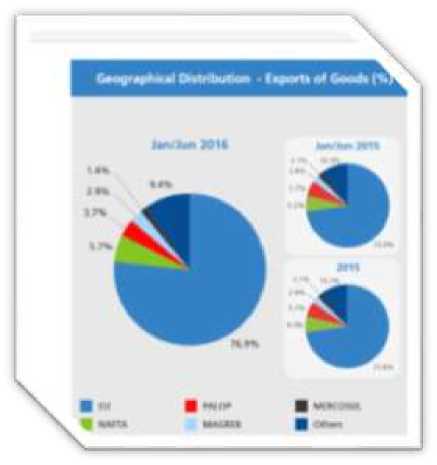
Picture 4. Goods Exports Geography.

Source: INE –National Statistics Office

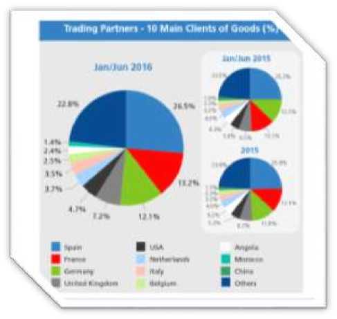
Picture 5. Main Clients. Source: INE - National Statistics Office

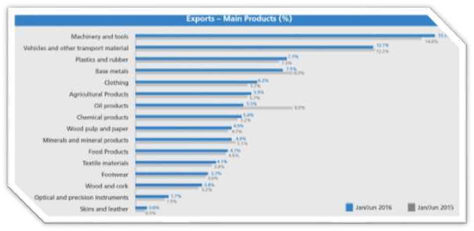
Picture 6. Exports – Main Products. Source: INE - National Statistics Office

In relation to the imports of goods, machinery and tools, vehicles and other transport material, chemicals and agricultural products and mineral fuels, lead the ranking in foreign purchases made during the 1st half 2016, representing 61.6%

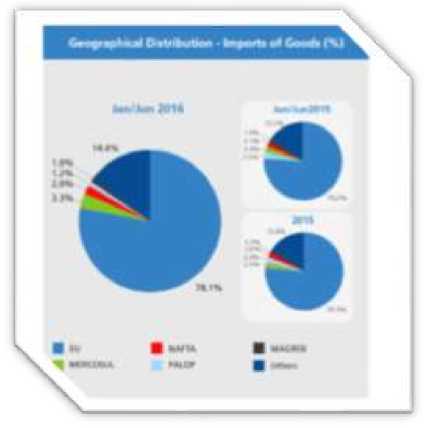
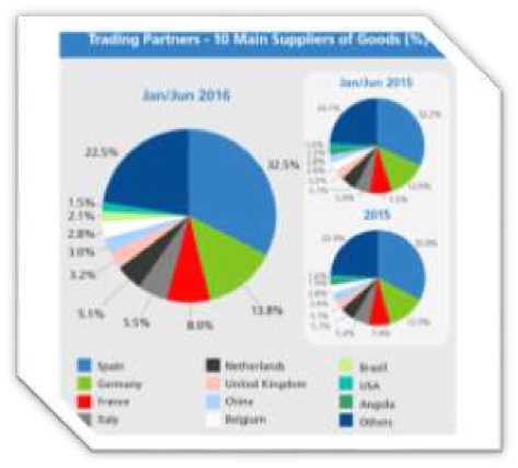
of the total (against 63.3% in the 1st half 2015) . The EU was the origin of the majority of imported products over this period with 78.1% of the total, followed by MERCOSUL (3.3%), NAFTA (2%), PALOP (1.2%) and MAGREB (1%). Spain, Germany, France, Italy and the Netherlands continue to be the main suppliers, together representing 64.9% of imports made during the 1st half 2016.

Picture 7. Goods Imports Geography. suppliers.

Source: INE –National Statistics Office

Picture 8. Main

Source: INE - National Statistics Office

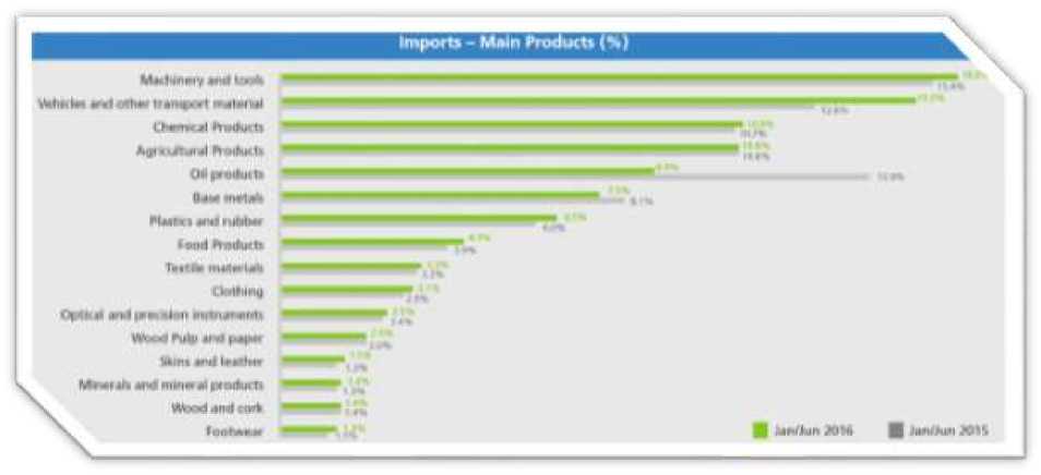
Picture 9. Imports – Main Products. Source: INE - National Statistics Office

International Investment

Foreign direct investment flow into Portugal (Directional principle)

According to data from the Banco de Portugal and the Directional Principle, the flow of Foreign Direct Investment into Portugal (FDI), in net terms, registered 15

an amount close to 5.4 billion Euros in 2015 (-5.1% in relation to 2014). The highest value in the last five years was registered in 2012, when FDI reached 6.9 billion Euros and in 2014 with 5.7 billion Euros.

In the 1st half 2016 the registered value of FDI was higher than 3.9 billion Euros (-33.5% in comparison to the same period in 2015).

Portuguese Foreign Direct Investment (PFDI), in net terms, was close to 4.5 billion Euros in 2015 (+47.5% in comparison to the previous year). The highest value during the period 2011-2015 was in 2011 (nearly 9.7 billion Euros).

In the 1st half 2016 PFDI value reached around 1 billion Euros (-76.7% in comparison to the same period in 2015).

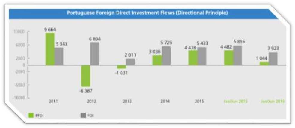
Picture 10. FDI Flows. Source: Banco de Portugal Unit: Million of Euros (net values) Note: Directional Principle: reflects the direction or influence investment, that is, Portuguese Foreign Direct Investment (PFDI) and Foreign Direct Investment in Portugal (FDI)

Portuguese external direct investment stock (Directional principle)

In terms of stock of Foreign Direct Investment (FDI) into Portugal, at the end of December 2015, 105.5 billion Euros (+7.5% in relation to the value in

December 2014) were registered. At the end of the 1st half 2016 the stock in FDI in Portugal totalled 109.3 billion Euros (+2.6% in relation to June 2015).

However, in relation to stock of Portuguese Foreign Direct Investment (PFDI) this represented close to 54.7 billion Euros in December 2015 (+11.6% in relation to December 2014). In June 2016 the stock of PFDI rose to nearly 55.8 billion Euros (+0.7% in relation to June 2015).

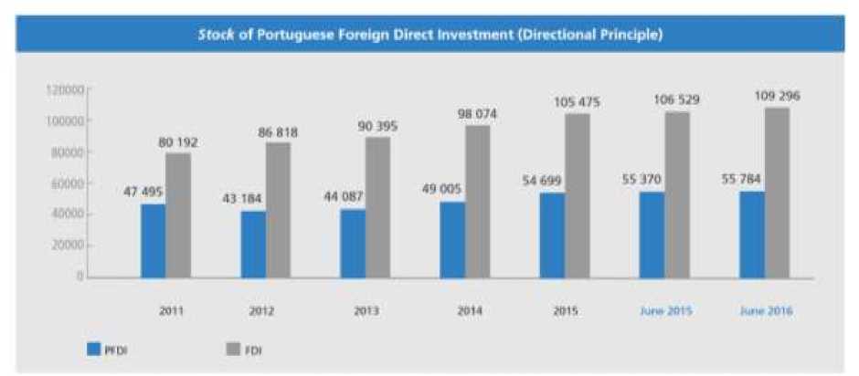
Picture 11. Stock of FDI. Source: Banco de Portugal Unit: Position at the end of the period in Million Euros Note: Directional Principle: reflects the direction or influence investment, that is, Portuguese Foreign Direct Investment (PFDI) and Foreign Direct Investment in Portugal (FDI)

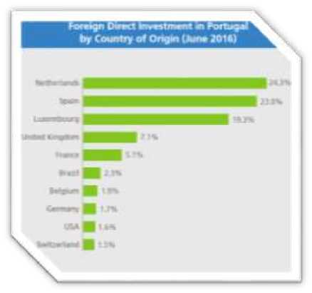
Foreign direct investment stock in Portugal by country of origin (Directional principle)

In global terms the European Union was the principle origin of FDI in Portugal, with a quota of 88% in June 2016, highlighting, on an intra-Community level, the Netherlands and Spain (with 24.3% and 23% of the total, respectively), Luxembourg (19.3%), United Kingdom and France (7.1% and 5.1% respectively). Within the non-EU countries (12% of the total), the following countries are highlighted: Brazil (2.3% of the total), the USA (1.6%), Switzerland and China (with quotas of 1.5% each).

Picture 12. FDI by Country of Origin. Source: Banco de Portugal Unit: Position at the end of June 2016 (% of the total)

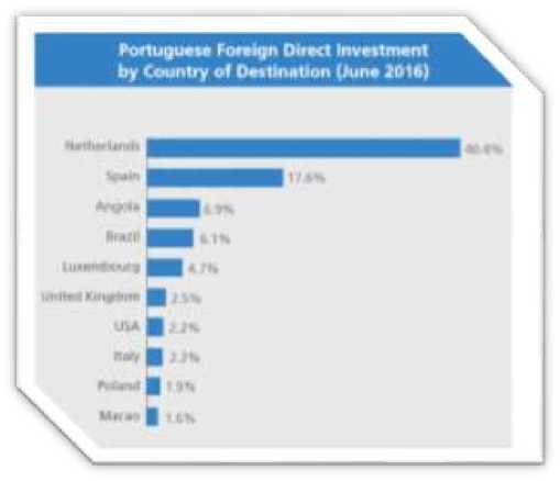
Portuguese foreign direct investment stock by country of destination (Directional principle)

The European Union was also the main destination of PFDI in global terms, with a contribution of 73.9% in June 2016, highlighting, on an intra-Community level, the Netherlands and Spain with quotas of 40.4% and 17.6% of the total, respectively, followed by Luxembourg with 4.7%. Within the non-EU countries (26.1% of the total in June 2016), the following countries are highlighted: Angola, Brazil and USA, with quotas of 6.9%, 6.1% and 2.2% respectively.

Picture 13. FDI by Country of Destination. Source: Banco de Portugal Unit: Position at the end of June 2016 (% of the total)

Tourism

In 2015, the Portuguese tourism trade balance was 7.8 billion Euros, having increased by 10.8% in relation to 2014.

According to the Banco de Portugal, tourism revenue in Portugal has seen a sustainable growth during the period 2011-2015, having reached an annual average increase of 8.9%. In 2015, revenue nearly reached 11.5 billion Euros (value that represents about 15.4% of the total Portuguese exports of goods and services), registering a significant increase of 10.2% in relation to the previous year.

In the 1st half 2016, tourism revenue registered an increase of 9.2% in relation to the same period of the previous year, reaching nearly 5 billion Euros.

The main markets generating tourism revenue to Portugal, in the 1st half 2016, were the United Kingdom (with 18.3% of the total), France (15.5%), Spain (13.2%), Germany (12%) and the Netherlands (4.9%), that together made 63.9% of the total for this period.

THE EMPIRICAL PART

This work investigates the relationship between a number of endogenous

(dependent) factors and exogenous (independent) ones.

Table 5. Variables Used

Variable	Description	Explanation	Unit of measure
Endogenous variables
M1 t	money supply for period t	M1 includes currency i.e. banknotes and coins, plus overnight deposits. M1 is measured as a seasonally adjusted Source: The Organisation for Economic Cooperation and Development	Index based on 2010=10 0.

ExtRes t foreign exchange reserves for period t Total reserves minus gold. Comprise special drawing rights, reserves of IMF members held by the IMF, and holdings of foreign exchange under the control of monetary authorities. Gold holdings are excluded. Source: International Financial Statistics (IFS) Millions of   US Dollars Exogenous variables GDP t Gross Domestic Product for period t Monetary measure of the market value of all final goods and services produced in a period Source: International Financial Statistics (IFS) Billions of Euros C t Consumpti on expenditure s for period t It consists of the expenditure incurred by resident    households    on    individual consumption goods and services Source: International Financial Statistics (IFS) Billions of Euros Exp t Export from Portugal for period t Selling goods and services produced in the home country to other markets Source: International Financial Statistics (IFS) Millions of   US Dollars

Source: International Financial Statistics (IFS)

The benchmark data collected are presented in table 6

Table 6. Benchmark data

'year'	M1'	'ExtRes'	'GDP'	'C'	'Exp'	'Imp'	'ST rate '	'LTrate '	'Debt'	'Aver ageE UR_ USD'
	Y	Y	X	X	X	X	X	X	X	X
1996	21,90	15917,66	93,09	60,82	25,36	32,04	7,37	8,56	101300,17	1,29
1997	25,30	15659,97	100,98	64,94	28,07	36,32	5,74	6,36	123205,30	1,13
1998	28,80	15824,62	110,10	69,84	30,82	41,04	4,31	4,88	165028,14	1,11
1999	33,10	8427,12	119,64	75,57	31,67	44,05	2,96	4,78	169163,44	1,07
2000	37,50	8908,69	128,47	81,26	36,22	50,40	4,39	5,60	197636,95	0,92
2001	41,50	9666,60	135,83	85,14	37,25	51,13	4,26	5,16	220904,93	0,90
2002	45,50	11179,11	142,63	89,27	38,43	50,23	3,32	5,01	286544,82	0,95
2003	51,00	5875,85	146,16	92,24	39,10	49,24	2,33	4,18	388761,17	1,13
2004	57,00	5174,07	152,37	96,80	41,53	54,11	2,11	4,14	458108,00	1,24
2005	64,80	3478,69	158,65	102,11	42,41	56,86	2,18	3,44	444064,56	1,24
2006	73,20	2063,64	166,25	107,30	49,74	63,43	3,08	3,91	556431,06	1,26
2007	79,20	1257,78	175,47	113,71	54,41	67,81	4,28	4,42	691413,33	1,37
2008	83,60	1309,40	178,87	118,49	55,67	73,05	4,63	4,52	659482,11	1,47
2009	91,50	2454,89	175,45	113,51	47,51	59,66	1,23	4,21	751399,13	1,39
2010	100,0 0	3651,91	179,93	118,33	53,75	67,35	0,81	5,40	716060,90	1,33
2011	104,1 0	1974,60	176,17	115,96	60,41	67,95	1,39	10,24	639408,82	1,39
2012	108,7 0	2196,02	168,40	111,61	63,50	64,36	0,57	10,55	690431,78	1,28
2013	117,8 0	2777,52	170,27	111,14	67,28	65,57	0,22	6,29	706896,13	1,33
2014	127,1 0	4869,35	173,08	114,06	69,36	69,03	0,21	3,75	648748,92	1,33

Correlation analysis

We have conducted the correlation analysis for the purpose of assessment the internal relationships between factors.

Correlation analysis typically gives us a number result that lies between +1 and -1. The +ve or –ve sign denotes the direction of the correlation. The positive sign denotes direct correlation whereas the negative sign denotes inverse correlation.

Zero signifies no correlation. And the closer the number moves towards 1, the stronger the correlation is. Usually for the correlation to be considered significant, the correlation must be 0.5 or above in either direction.

The most significant correlation of ExtRes can be observed with the GDP factor, stated for -0,943. Simultaneously, The most significant correlation of M1 can be traced with Exp factor, for 0,978.

Table 7. Correlation analysis

	M1'	ExtRes '	GDP'	C'	Exp	Imp	STrate	LTrate	Debt	Average EUR_US D'
M1'	1,000
ExtRes'	-0,801	1,000
GDP'	0,885	-0,943	1,000
C'	0,907	-0,938	0,997	1,000
Exp'	0,978	-0,805	0,878	0,898	1,000
Imp'	0,891	-0,912	0,969	0,975	0,918	1,000
STrate'	-0,808	0,674	-0,730	-0,721	-0,749	-0,657	1,000
LTrate'	0,141	0,081	-0,100	-0,052	0,150	-0,050	0,007	1,000
Debt'	0,930	-0,899	0,956	0,969	0,901	0,922	-0,719	0,018	1,000
AverageEUR_U SD'	0,679	-0,609	0,616	0,662	0,627	0,609	-0,324	0,144	0,764	1,000

SYSTEM OF EQUATIONS

For the analysis, a system of interrelated linear equations was made ln(M1) = a1+b11*ln(GDP)+b12*ln(C)+b13*ln(Exp)+b14*STrate + e1 equation 1

ln(ExtRes)=a2+b21*ln(M1)+b22*ln(Imp)+b23*ln(ExRate)+b24*ln(Deb t)+b25*LTrate+e2 – equation 2

where,

Equation 1

ln(M1) = a1+b11*ln(GDP)+b12*ln(C)+b13*ln(Exp)+b14*STrate + e1

The assumption of the suggested equations system is that the analyzed economic factors can be approximated by a log-normal distribution. Further on, the testing of the hypothesis is provided.

Taking the logarithm of a factor when constructing a linear regression model minimizes the relative (not absolute) deviation from the regression line.

The given system of equations belongs within the recursive type, since the endogenous factor M1 from the first equations at the same time serves as the explaining factor for the second equation.

Thus occurs the following mechanism of assesing the model parameters:

The first step provides estimates of the parameters of equation 1, and as a result of the estimated model we obtain M1 theoretical values estimation (the values are unbiased).

Further on, the above mentioned values are used to assess the parameters of equation 2 during the second stage of the recursive equations system identification.

STEP 1 OF 2 OLS

Estimation of the parameters of the given form of model in relation to the endogenous ln(M1)

ln(M1) = a1+b11*ln(GDP)+b12*ln(C)+b13*ln(Exp)+b14*STrate + e1

Linear regression model (scheme) from MATLAB:

lnM1~1+lnGDP+lnC+lnExp+STrate

Table 8. F-statistics

Number of observations	19
Error degrees of freedom	14
Root Mean Squared Error	0.0407
R-squared	0.996
Adjusted R-Squared	0.995
F-statistic vs. constant model	820
p-value	1.99e-16

The regression relation significance is shown by p-value of dispersion analysis (F-statistics). The null hypothesis that R2=0 has been rejected, therefore, the model is significant. The value of R2 is high (R-squared = 0.996).

Using the coefficients of the regression model the following statistical results are obtained:

Table 9. t-statistics

	Estimate	SE	tStat	pValue
(Intercept)	-1.6369	0.55337	-2.9581	0.010379
STrate	-0.054972	0.0082429	-6.6691	1.0626e-05
lnGDP	-3.2546	0.72353	-4.4982	0.00050089
lnExp	0.70304	0.11617	6.0517	2.9787e-05
lnC	4.2762	0.76433	5.5947	6.6078e-05

According t-test (student statistics), all factor’s coefficients are relevant (p-value<0.05), hence we should not exclude any of it from the regression equation.

As a result of analysis the repression equation is as follows:

ln(M1) = – 1.6369 – 3.2546 *ln(GDP)+ 4.2762 *ln(C)+ 0.70304 *ln(Exp) – 0.054972 *STrate

In order the F and t criterial were valid, it is obligatory that the values of our variables were distributed normally.

As calculated values are the logariphms to the factors, it means that our factors are distrubuted log-normally.

First and foremost, let us conduct the non-parametric test of Colmagorov-Smirnov. The findings are below.

Table 10. Kolmogorov-Smirnov test

Type of output	Values	Clarification of the output values
Ksstat (Kolmogorov-Smirnov statistics)	0.1122	Test statistic nonnegative scalar value Test statistic of the hypothesis test, returned as a nonnegative scalar value. The one-sample Kolmogorov-Smirnov test is a nonparametric test of the null hypothesis that the population cdf of the data is equal to the hypothesized cdf. The two-sided test for "unequal" cdf functions tests the null hypothesis against the alternative that the population cdf of the data is not equal to the hypothesized cdf. The test statistic is the maximum absolute difference between the empirical cdf calculated from x and the hypothesized cdf: D' = max( F(x) - G(x) ) X where ˆF(x) is the empirical cdf and G(x) is the cdf of the hypothesized distribution.

Сv (critical value)	0.3014	Critical value is a nonnegative scalar value Critical value, returned as a nonnegative scalar value.
p-value	0.9489	P-value scalar value in the range [0,1] p-value of the test, returned as a scalar value in the range [0,1]. p is the probability of observing a test statistic as extreme as, or more extreme than, the observed value under the null hypothesis. Small values of p cast doubt on the validity of the null hypothesis.
h	0	h — Hypothesis test result 1 | 0 Hypothesis test result, returned as a logical value. If h = 1, this indicates the rejection of the null hypothesis at the 0,05-significance level. If h = 0, this indicates a failure to reject the null hypothesis at the 0,05-significance level.

The findings show that the hypothesis of normalcy of distribution can be accepted (h = 0).

Hence, we can claim that the M (money supply) meets long-normal distribution.

Hence, we can conclude that the previous tests results (F-test, t-test) were relevant.

Normal probability plot of residuals is depicted on graph № 4

Graph 4. Normal probability plot of residuals

Mutmai ptobabtiCy plot of rttMuate

$W,.-'

О» Г^

07В г*                                                                 . *^ *

1“. ^”'

0 • ft Ci

•OB         4)M         nW          0          MS         104         QM         Ott          Bl Raaiduata Table 11. Durbin-Watson test
Type of output	Values	Clarification of the output values
DW	2.1665	Durbin-Watson test statistic The test statistic for the Durbin-Watson test is S Чл-Р2 where T is the number of observations, and et is the residual at time t.
P	0.4307	The p-value for the Durbin-Watson test of the null hypothesis that the residuals from a linear regression are uncorrelated. The alternative hypothesis is that there is autocorrelation among the residuals.

The p-value of the Durbin-Watson test is the probability of observing a test statistic as extreme as, or more extreme than, the observed value under the null hypothesis. A significantly small p-value casts doubt on the validity of the null hypothesis and indicates correlation among residuals.

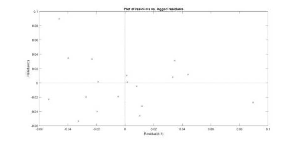
In order to verify residuals for the presence of auto regression, the Durbin-Watson test was conducted.

The findings showed that DW= 2.1665. P-value = 0.4307> 5%, which means that test is negative – the autocorrelation doesn’t exist.

Graph 5. Plot of residuals vs. lagged residuals depicted on graph

Adequacy verification

When verifying the model adequacy, the unselected data are being checked. In the capacity of such data, the indicators of 2015 have been used to analyze the deviation of theoretically predicted response from the actual one. In other words, the analysis verifies, whether the practical value of the response coincides with 95% of the confidence interval constructed around the theoretically predicted value. In case the value lies inside this interval, one can say that the model is adequate.

The indicators values for 2015 are given in table 12.

Table 12. Adequacy verification

	Y	X	X	X	X	X	X	X
'year'	'M1'	'GDP'	'C'	'Exp'	'STrate'	'lnGDP'	'lnC'	'lnExp'
2015	144,5	179,54	117,82	72,81	-0,02	5,190398	4,78	4,287853

'year'	Fact lnM1	Calculated value	Conf.int 95% min	Conf.int 95% max
2015	4.973279507552487	4.9264	4.8749	4.9780