The influence of slenderness ratio and stress concentration in taps on load calculations to thermal expansion in U-shaped compensators of thermal network

Author: Lipovka Yuri L., Belilovets Vitaliy I., Lipovka Alex Y.
Journal: Журнал Сибирского федерального университета. Серия: Техника и технологии @technologies-sfu
Article in issue: 1 т.8, 2015.
Free access
This article is about calculations of U-shaped regions of water heat network. The universal calculation algorithm is used for various geometric schemes and simple self-compensating pipeline sections. The influence of slenderness ratio and stress concentration factor in the smooth curved bends on voltages and maximum permissible flight compensated shoulders of U-shaped regions for different geometric confi gurations was taken into account in this work.
Radial u-shaped compensator, radial compensators, self-compensation for thermal expansion of pipeline, slenderness ratio of pipe, heating network
Short address: https://sciup.org/146114925
IDR: 146114925 | UDC: 697.443.3
Влияние коэффициентов гибкости и концентрации напряжения в отводах на расчет нагрузки от температурных расширений в П-образных компенсаторах тепловой сети
В настоящей статье рассматривается вопрос расчета П-образных участков водяной тепловой сети на самокомпенсацию температурных расширений. Приведен универсальный алгоритм расчета, применимый для различных геометрических схем простых, плоских, неразрезных самокомпенсирующихся участков трубопровода (Г-, Z-, П-, Л-образные конфигурации). Изложено влияние коэффициента гибкости и коэффициента концентрации напряжений в гнутых гладких отводах на значения напряжений и на предельно допустимый вылет компенсируемых плеч П-образных участков различных геометрических конфигураций.
Text of the scientific article The influence of slenderness ratio and stress concentration in taps on load calculations to thermal expansion in U-shaped compensators of thermal network
The most vulnerable elements in the radial compensators of pipeline are taps. The cross-sectional pipe wall ovalisation and increasing ductility in bending as compared with straight pipes appear in taps. Taps are pipeline’s elements with sharp change in shape. This change leads to a concentration of additional stresses in these elements arising under the influence of forces, their flattened crosssection.
Calculation model radial compensator, based on the thermal expansion, can be represented as a rod frame with rigid corners. In this case the taps geometry, their flexibility and concentration of bending stresses in them are not taken into account. Differences in results with calculated model, which reflects features of taps, are relevant.
The article has three computational models U-shaped pipe sections with aboveground way laying in the horizontal plane. There are following assumptions: pillars are absolutely rigid, resistance to friction forces movable bearings in longitudinal thermal expansion of pipeline is not considered.
Materials and Methods
When calculating pipeline to compensate radial thermal expansion compensators are determined their dimensions, in which longitudinal bending stresses arising from the elastic deformation of pipe will not exceed the permissible values. Rod model (pipeline’s length exceeds the outer diameter of more than an order of magnitude) is used as a design scheme of pipeline. П-shaped radial compensator is a simple (line called simple if it throughout its length from one to the other fixpoint has no branches) and a flat (line called flat if the center line is located in the same plane) plot calculated self-compensating pipe fixed between two fixed pillars. Computational model of this pipeline’s section under the influence of stress is a statically indeterminate system. Statically indeterminate system is called such a system in which the action of arbitrary load not all longitudinal and transverse forces and moments can be found from the equations of equilibrium of a rigid body or a solids system. Additional equations, which should express conditions of strain compatibility system, are introduced for calculations. Statically indeterminate system is characterized with number of extra links that is the largest number of links that can be removed at the same time without disturbing the geometric immutability and immobility system. In order to obtain additional equations, it’s necessary to select a base system. To achieve this goal n-defined statically indeterminate system is transformed into a statically determinate with removing unnecessary links from it. The resulting system is called statically determinate basic. Elimination of any links does not change internal forces and deformation of the system, if it makes additional forces and moments, which are the reaction dropped connections. Thus, if you apply a given load and response remote connections to basic system, this and considered systems will be equivalent. In considered system the directions of available hard links, including those relationships discarded in the transition to basic system, there can be no movement, and therefore in basic system moving in the – 12 – directions of dropped connections must be zero. And for this reaction must have dropped connections strictly defined values. Zero movement condition in the direction of any i-th connection of n-dropped on basis of the superposition principle has the form
Д;= ^ Aik + Д№= 0, (1)
Р(Ю where Aik - movement in the direction of i-th communication system caused by the reaction of the k-th connection;
Д,р - movement in the direction of i-th communication system caused by the simultaneous action of all external load.
In the method of reaction forces k-th connection usually denoted Xk. With this notation, and in the power of Hooke’s law movement ^ t k can be written as
^tk= 8ikxk, (2)
where otk - single (or specific) moving in the direction of i-th communication system caused by the reaction of Xk - 1, i.e. reaction, which coincides with the direction of Xk, but unity.
Substituting (2) into (1), we obtain
^^=0 (3)
p(k)
The physical meaning for equation (3): moving in the direction of basic system i-th dropped connection is zero. Writing expressions, similar to (3), for the entire set of dropped connections, we obtain the system of canonical equations force method, which can be represented as a single equation
.
The total number of terms is determined with degree of the system’s redundancy and does not depend on its specific characteristics. Single movement system is determined according to next formula
V Г -MM..
"k L' к dL where 5^ – single movement of the i-th direction, caused by a single exposure, applied at the point k;
M i - bending moment from a single exposure, applied at the point i;
Mk - bending moment due to impact of the unit applied to the point k;
K – slenderness ratio element;
v – basic element stiffness to element’s stiffness;
l - integrable element length.
The main problem of calculation for pipeline as a statically indeterminate system is formulated as follows: for a given geometric scheme, the temperature difference between hot and cold pipeline and size of pipes constituting portion is required to determine the effort and strain the system. In – 13 – calculating the temperature effects on simple pipelines as the main unknown is usually accepted in forces and moments of extra links, and therefore, this method is called the method of calculating forces. According to the method forces, one of the fixed pillars calculated area is considered breakout, and it’s applied to elastic deformation forces and bending moment replacing a dropped pillar.
To determine elastic forces arising in pipeline with thermal expansion, the authors use the method of the elastic center. This method is well considered in [1, 2] and presents one of modifications of the force method, which consists in the fact that all side coefficients of canonical equations (i.e., coefficients δ ik , in which i ≠ k) become zero. This is achieved by moving basic unknowns of fixpoint dropped into the elastic center of gravity calculated of pipeline. The application point for basic unknowns is connected to the point of placing a dropped pillar infinitely rigid hypothetical console. The pipeline’s axis will be endowed with a certain distribution of the elastic mass proportional to its stiffness (Fig. 1).
Bending moment from forces of elastic deformation in any section of pipeline is determined with the formula
M = (y-y0)Px-(x-x0)Py,
where x , y – coordinates of considered section in the original coordinate system;
x 0 , y 0 – coordinates of gravity center calculated elastic pipeline section;
P x , P y – elastic forces calculated center line of pipeline.
The basis for calculating the forces of elastic deformation has been put the Castigliano’s theorem. Load is static and strain energy equal to work of external forces
dU
ь, = а7/
л
dU лу=^^/
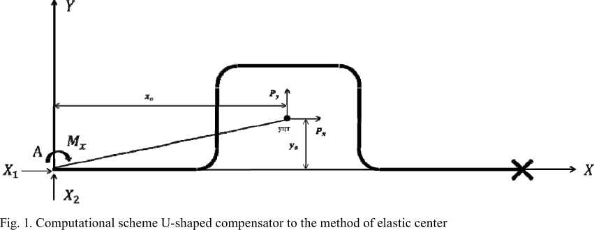
Note: X 1 , X 2 , M x – longitudinal and transverse forces and bending moment respectively; А – the application point force and moment, replacing the dropped fixed pillar; уцт – the point elastic center of gravity of the system with respect to coordinate; P x , P y – vectors elastic forces relative to the coordinate axes X and Y, respectively; x 0 , y 0 – coordinates of the elastic center of gravity relative to the coordinate axes X and Y, respectively.
here U – strain energy;
P x , P y – the same, in the formula (6);
Δ x , Δ y – displacement for the application point of force in its direction along respective axes. Displacement Δx, Δy calculated thermal extensions
Lx = aMLr,
Л
Ду = a^tLy, where α – coefficient of linear thermal expansion;
Δ t – design temperature drop;
Lx , Ly – lengths of axial line section of projections on axes.
Values of the basic unknown P x = X 1 , P y = X 2
p = rx
^X] yO + ^y] xyO „ - htJ J xo j yo J xyo
_ л^/. + ^X]xyo c r
— r r r 2 ^tJ
Jx0Jy0 -Jxy0
where Δ x , Δ y – calculated thermal expansion of area under consideration conduit in the direction x and y axes, respectively;
Et – modulus of elasticity the pipe material at the calculation temperature;
J – inertia moment of the cross section of pipe wall
H
/ = ^[Ян4-(Ян-25П (13)
where D н – outer diameter of pipeline;
δ – pipe wall thickness;
Jx0, Jy0 – central inertia moments of the reduced length for the centerline of pipeline section
K – the same, in the formula (5);
Jxy 0 – central centrifugal inertia reduced length for the centerline of pipeline section
J xyO
-I
xyds ПГ
-х о У о
f ds
Jt
Stiffness reduction factor is introduced in integrating along the curved pipeline sections, so here straights K = 1, and for curved K <1.
Elastic center coordinates can be determined from equations
^5
% о
SxT_sy
J^ Lnp r ds м J У К _ Уо" rds "L„p J К where Sx, Sy – static inertia moments of reduced length for the centerline of calculated pipeline section relative to x and y axes, respectively;
L пр – reduced length of axial line section.
Karman researches have shown that the curvature bends causes ovalisation their original crosssectional area and stiffness reduction. Flattening of initial round section causes essential changes in distribution of bending stress compared with bending solid beams. To determine the coefficient of flexibility Karman used the energy method, followed by a solution of the Ritz method. The decision was received in form of trigonometric series. It is alleged that results obtained by T. Karman significantly diverged from the experimental data. Note that in the derivation of the coefficient of flexibility in order to facilitate mathematical calculations Karman made a number of assumptions and, in particular, he disregarded pipe radius relation to bend radius, considering this relationship as a very small amount. He also did not consider displacement of the neutral layer. Reported assumptions may be valid only for a relatively small pipe curves of curvature, i.e. a larger radius of curved (4 – 5 outer diameter) [3]. At the moment the calculating problem of pipe elbows has produced many works. For example, in [4, 5] there are analytical solutions for curves pipes. Materials [6, 7] are devoted to solution curves of pipes using the finite element method.
Karman coefficient for curved smooth retraction we calculate according to [8]
К = 1/(Kp^),
where Kp – slenderness ratio, excluding constraint deformation ends of the curved portion pipeline kp
1,65 л^Г
here λ – geometric characteristic flexibility removal л =
4R8
ФТ-зу-
where R – radius of curvature for tap;
D н ,δ – the same, in the formula (13); ω – dimensionless parameter
PR^
ш = 3-64^ТБ ---- Et(DH - 5)5
where P – excess internal pressure in pipeline;
R – the same, in the formula (21);
D н ,δ – the same, in the formula (13);
E t – the same, in the formula (11);
ξ – coefficient reflecting the uneasiness of deformation at the ends of curved element (tap), at λ ≤ 1,65 calculated with the formula
-
<-Т^ + *“-*"<*-1^] ' (23)
here ψ – angular parameter
^ = ^2R/(DH-s), (24)
where R – the same, in the formula (21)
D н ,δ – the same, in the formula (13);
-
ϑ – central angle of tap in radians.
When λ > 1,65 value for ξ is set equal to 1.0. Slenderness ratio bent pipe with straight sections at the ends with λ > 2,2 is 1.0, while λ ≤ 2,2 is calculated with formula (19).
When bending tap under the influence of forces, flattened their cross section, there are significant local stresses. If longitudinal stresses, calculated in the usual theory of bending, are denoted by σ, then the maximum longitudinal stresses can be determined with the formula a— = ioa, (25)
where i – concentration ratio of longitudinal stresses in tap;
l ° = t^^ , (26)
where λ – the same, in the formula (20).
9-element model pipeline section
Calculation algorithms to compensate for thermal expansion of pipeline sections certain geometric configurations are presented in references for design of heat networks in section strength calculations. If you submit a calculation algorithm based on using a certain number of standard elements that are building design model, the resulting algorithm is applied to self-compensating schemes pipelines of various geometric configurations. Further, consider the scheme of 9 elements. This circuit includes straight 5 pipes and 4 of the same smooth curved drainages random rotation angle. We give as an illustrative example П-shaped pipeline section between two fixed pillars. Mentally divide it into nine elements: five straight pipes and four identical taps. The following is an algorithm based on self-compensation for thermal expansion of sector and its design scheme. This algorithm may be applied to other design schemes by removing unnecessary components, changes in steering angle taps (Fig. 2).
Elements l 1, l 3, l 5, l 9 are parallel to the coordinate axis X.
Distance from ends of curved element (tap) from its center of gravity in the direction of the reference coordinate system, according to design scheme of curved element (Fig. 3), determined by the formula
a = R [sin^sin^ + Usiny- У cos уА^0^ 57,296
2 2 57,296 2 у .
b = R
sin У sinp - (2sin У - У cos У) C0S^ 57,296 2 2 57,296 2 у .
c = R
" . Ф Ф
sm2cosp -^2sm2-
57,296
Ф
C0S 2)
sinB
—- 57,296l,
Ф
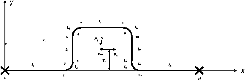
Fig. 2. Calculation scheme 9-element П -shaped pipeline section
Note: numbers on the diagram below to identify numbers of sections; уцт – elastic center of gravity; l 1 , l 2 , l 3 ,…, l 9 elements of calculated area; P x , P y – elastic resistance forces (basic unknowns); x 0 , y 0 – distance from the center of gravity and elastic axes.
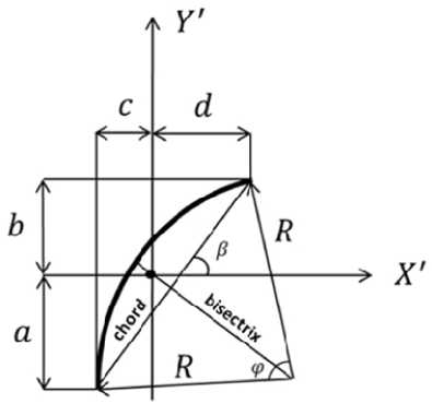
Fig. 3. Calculation scheme curved element (tap)
Note: a,b,c,d – distance from ends of the curved element (tap) to its center of gravity; R – radius of tap’s curvature; φ – central angle of tap; β – chord angle curved element (tap) to its axis of ordinates.
d = R
[sm | cosp + (2sin ^) ^ 57,29б1,
[ 2 p V 2 57,296
where angles φ , β are measured in degrees.
Projection lengths taps on the coordinate axes are defined as
Per axle x
Ltx = c + d,(31)
where c, d – the same, in the formula (27) and (28);
i – tap number (index takes values 1, 2, 3, 4). Per axle y
Liy - a + й , where a, b – the same, in the formula (29) and (30);
i – the same, in the formula (27).
The length of the axial line for calculated total pipe section is determined by the formula
К – the same, in the formula (19).
Center coordinates of gravity of individual elements, according to calculation scheme area (Fig. 2) with respect to the x-axis defined by the formulas
Relative to the axis x
|
Z 1 xcl=2, |
(35) |
|
xc2 = l1 + d , |
(36) |
|
-1 ^1/ C3 1 lx 2 3 |
(37) |
|
X c4 -h + Llx + l3 C 0SV + C , |
(38) |
|
1 %c5 - Z1 + L 1X + 13CO^) + L3x + 2l3, |
(39) |
|
Xc6- l i + L i x + l 3 COSV +L3x + l 3 +d , |
(40) |
|
1, X c ? - 1 1 + L 1x + l 3 C0 S ) + L ^ x + l s + L 3x + 2 l 7 C0S) , |
(41) |
' L- г .. - 1 г°°^, ■ L . ■ l ■ L . ■ Уг,.^, + Г . (4 2)
X = к + Llx + 13СО8Ф + L . + Z5 + L . + 17созФ + L 4X + |Z9, (43)
Relative to the axis y
1,
,44,
'(45)
у =L +-151ПФ(46)
-
i, 2
W yc6 = Lly + 1381Пф + a,(49)
Ус7=Ь1, + 1з51Пф-21751Пф,(50)
У18 = 11, + 1зУ,„ф-|7.Пф-а, yc9 = 1381Пф - 1781Пф,(52)
where x c 1 – x c 9 ; y c 1 – y c 9 – section elements;
-
l 1, l 3, l 5, l 7, l 9 – length for corresponding calculation scheme (Fig. 2) elements;
L 1 x – L 4 x – the same, in the formula (31);
L 1 y , L 2 y – the same, in the formula (32);
-
a , b , c , d – the same, in the formulas (27) – (30);
φ – the same, in the formulas (27) – (30).
Static inertia moments of length pipeline components in original coordinate system, according to calculation scheme area (Fig. 2), are determined by formulas
Relative to the axis x
Sx! = ^1Ус!>
Sx. = ?отвУс2,
Sx3 = 1зУсз,(55)
Sx4-l°TB,„.,56)
-
5 .5 IsVcS,
Sxg = ктвУсб,(58)
-
l 1 , l 2, l 3, l 4, l 5, l 6, l 7, l 8, l 9 – length for corresponding calculation scheme (Fig. 2) elements;
l отв – the same, in the formula (34).
Coordinates elastic center of gravity relative to origin of the coordinate system according to calculation scheme area (Fig. 2) have the following form
The axis х
S x 1 – S x 9 – the same, in the formulas (53) – (61);
L пр – the same, in the formula (33).
Coefficients for calculating inertia moments of its own elements 3 and 7 of the calculation scheme area (Fig. 2) relative to initial coordinate system defined by the formulas
The axis х
C xi
sin2^
12 '
The axis у
cos2ф
Cyl = ""12-'
where φ – the same, in the formulas (27) – (30).
Factor to calculate the inertia moment of its own centrifugal element 3 the calculation scheme area (Fig. 2) relative to the initial coordinate system is calculated by the formula
sin^cos^ Cxyl(3) = 7^ ,
where φ – the same, in the formulas (27) – (30).
Factor to calculate the inertia moment of its own centrifugal element 7 the calculation scheme area (Fig. 2) relative to the initial coordinate system is calculated by the formula
51ПфС05ф
Cxyl(7) = 12
where φ – the same, in the formulas (27) – (30).
Coefficients for calculating inertia moments of its own curvilinear elements (taps) relative to the initial coordinate system defined by the formulas
The axis х
C,2 = ^572964siЛ2ф-sinф)siЛ2^+1sinф-572964sin
\ Ф 2 ) 2 Ф
2^ +___Ф___ 2 2(57,296) ,
The axis у
CУ2 = (57.296^sin22-sinф)COs2^+lsinф
Ф
Ф
57,2964 sin2 ^ + ,
Ф 2 2(57,296)
where φ, β – the same, in the formulas (27) – (30).
Coefficients for calculating inertia moment of its own centrifugal curvilinear elements 2 and 4 of the calculation scheme section relative to the initial coordinate system is calculated by the formula
Cxy2(2;4) = (57,2964sin2 Ф - Sinф^ sin^cos^, k v Ф 2 /
where φ, β – the same, in the formulas (27) – (30).
Coefficients for calculating inertia moment of its own centrifugal curvilinear elements 6 and 8 of the calculation scheme section relative to the initial coordinate system is calculated by the formula
CXy2(6;8) = - (57,296 —sin2 2 - sinф^ sin^cosp,
where φ, β – the same, in the formulas (27) – (30).
Inertia moments of element lengths for pipeline in the original coordinate system relative to the x-axis are determined by formulas
The axis х
7„=l 1( l , 2
sin2(0°)
+yc,=).
JX2=^(R2CX2+yc22r^\-
К V 57,2967
Jx3 = l3(l32Cxl + yc3^),
,=R(R2r„ + _^L_\ к I 57,296)
.„.-Gt
V
sinW
+ уЛ
_R / 2 2 ф \
КI 57,2967
Jx7 = l7(l72Cxl+yc7^),
Lo=^fff2C,+y 2^^
КI 57,296/
I -lG 2 7„-1, l,
stn2(0°)
\
+ yC92j,
where J x 1 – J x 9 – section elements;
R – the same, in the formulas (27) – (30);
К – the same, in the formula (19);
y c 1 – y c 9 – the same, in the formulas (44) – (52);
l , l , l , l , l – length for corresponding calculation scheme (Fig. 2) elements;
φ – the same, in the formulas (27) – (30);
C x 1 – the same, in the formula (73);
C x 2 – the same, in the formula (77).
The axis у
J" l,(l,2
cosW
+ X„2),
_R/ 22
/y2 K^R Cy2+Xc2 57,296J'
2Г2)
h3 - ^U3 Lyl +Xc3 ),
^
у КI y 57,296.
2 <™ 2 (0 ° )
12}
R^ Ф
/У6 K^R С у2 + %с6 57 , 296) ,
Jy7 = l7(l72Cyl+Xc72),
^(^Л^ (97)
/у9 — Z 9
( .COS2^
V9 12
+ % с9 2 ) ,
where Jy 1 – Jy 9 – section elements;
R – the same, in the formulas (27) – (30);
К – the same, in the formula (19);
x c 1 – x c 9 – the same, in the formulas (35) – (43);
-
l 1, l 3, l 5, l 7, l 9 – for corresponding calculation scheme (Fig. 2) elements;
φ – the same, in the formulas (27) – (30);
C y 1 – the same, in the formula (74);
C y 2 – the same, in the formula (78).
Centrifugal inertia moments for length of pipeline components in the original coordinate system (Fig. 2) are determined by formulas
|
_ ( 2sin(0 ° )COs(0 ° ) \ 7*yl " 11 V* 12 + Х с, У с1 } |
(99) |
|
У2 К ' ' У2( ’ ’ 5729 |
(100) |
|
J ^ ^.. 1 +х . . |
(101) |
|
R / _ Ф \ Ay . - K ( R c .y2 <„, + xc.y^ |
(102) |
|
7 , <,2 sin(0 ° )COs(0 ° ) , \ х у 5 5^5 12 Хс5ус5), |
(103) |
R(mrФ
Jxy 6 - K ( R С . у2( 6^) + % с6 у сб 57,296),
Ьу7 = 17(17Ху1(7)+хс7У^(105)
R(^r
Jxya к (R СЖу2(6:8) + хс8ус8 57,296/ ’
( 2sin(0o)cos(0o) \
Jxy9 ^9 I ^9 12 + ^с9Ус9 I , where Jxy1 – Jxy9 – section elements;
R – the same, in the formulas (27) – (30);
К – the same, in the formula (19);
x c 1 – x c 9 – the same, in the formulas (35) – (43);
y c 1 – y c 9 – the same, in the formulas (44) – (52);
-
l 1, l 3, l 5, l 7, l 9 – for corresponding calculation scheme (Fig. 2) elements;
φ – the same, in the formulas (27) – (30);
Cxy 1 ( 3 ) , Cxy 1 ( 7 ) – the same, in the formulas (75) and (76);
C xy 2(2;4) , C xy 2(6;8) – the same, in the formulas (79) and (80).
Central inertia moments calculated for total length of pipeline relative to the axis passing through the elastic center of gravity, according to calculation scheme area (Fig. 2) calculated by the formulas
The axis х lxo = ^ki - ^прУо2,
1 1
Th eaxis у lyo=^lyt-LnpXo2,(109)
i=i where J – the same, in the formulas (81) – (89); xi
J yi – the same, in the formulas (90) – (98);
L пр – the same, in the formula (33);
x 0 , y 0 – the same, in the formulas (71) и (72).
Central centrifugal inertia moment total calculated pipeline section relative to the axis passing through the elastic center of gravity, according to calculation scheme section (Fig. 2) is defined as
I xyO — ^/ xyi
Ь пр Х о У о ,
where J xyi – the same, in the formulas (99) – (107);
L пр , x 0 , y 0 – the same, in the formulas (33), (71), (72).
Calculated temperature elongation for total calculated pipeline section are determined by formulas
The axis х
^Х — E^(t1 t2)(li + LTx + 13СО5ф + L2x + Z5 + L3x + 17С05ф + L4x + ?9), (111)
The axis у
Ду = eA(t1 - t2)(Lly + 13з1пф + L2y - L3y - 17з1пф - L4y), (112)
where ε – primary pipeline stretching coefficient;
A – linear thermal expansion of piping material at an estimated coolant temperature (pipe wall);
-
t 1 – calculated coolant temperature (pipe wall);
-
t 2 – installation temperature;
-
l 1, l 3, l 5, l 7, l 9 – for corresponding calculation scheme (Fig. 2) elements;
L 1 x – L 4 x – the same, in the formula (31);
L 1 y , L 2 y – the same, in the formula (32);
φ – the same, in the formulas (27) – (30).
Distance from the gravity’s center of the arc for the curved element (tap) to the center of curvature along the bisector (Fig. 3) is determined by the formula
7srn^
р = 57,296----2R, (113)
Ф
Bending moments in cross sections at ends of linear elements and in the middle taps according to calculation scheme area (Fig. 2) are determined as
М1 = -УоРх + хоРу ,
|
2 У о x ( 1 о) у , |
(115) |
|
*-\»-^Н р х |
- \l i + d + (R - p) cos 2 -x „ ]P y . (116) |
|
M4 = (llv- y „ ) P , - (l 1 + L1 , - |
x0X , (117) |
|
M 5 = (L i y + l 3s i n v - У о )Р х - (h + L 1 X + l 3cos v - x 0)P y , |
(118) (119) (120) |
|
|
Ф 6 I 1y 3 2 2 — \l+L + lC 0 S V + C- (R - p) C0S^- X 2 М7 = ( £ 1 у + ^+ £ 2у-У ° ) р х - -(Z 1 + L1x + Z 3c os . + L 2x - X ° ) py , |
- У „ ] р х - -x „ ] p y , |
|
|
( ) 8 1 y 3 ^ 2 y У ° x -( Z 1 + L 1x + ? 3 cos ^ + L 2x + ? 5 - X ° )P y , |
(121) |
|
Ь + L + ; cos
[ 1 lx 3 2x 2 °J y '
'. .P
..-,
P x , P y – the same, in the formulas (11) and (12);
-
l 1 , l 3 , l 5 , l 7 , l 9 – for corresponding calculation scheme (Fig. 2) elements;
L 1 x – L 4 x – the same, in the formula (31);
L , L – the same, in the formula (32); yy
φ – the same, in the formulas (27) – (30);
ρ – the same, in the formula (113);
x 0, y 0 – the same, in the formulas (71) and (72).
Section modulus of the pipe wall defined as
D н – the same, in the formula (13).
Bending compensation voltage in the i-th section, according to calculation scheme area (Fig. 2), determined by the formula
W – the same, in the formula (128).
Results of research for computational models of U-shaped compensators
Consider three computational model U-shaped compensators located in the horizontal plane and are not clamped by the ground. For each computational model variate is the radius of curvature tap. Please find enclosed characteristics of computational models below. In calculations of fixed points were considered to be absolutely rigid and do not take into account the resistance of friction forces movable pillars.
Table 1. Characteristics of computational models U-shaped compensators
। allowable stress for the section in the horizontal plane
-
-*- allowable stress for the section in the vertical plane
rated voltage (excluding the impact of taps geometry, flexibility and coefficients of
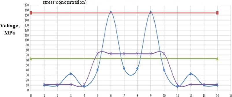
Fig. 4. Graph of stress distribution compensator number 1 at radius of the outer diameter of tap pipe to one
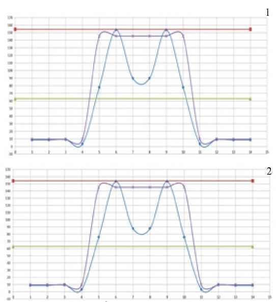
Fig. 5. A graph of voltage compensator number 1 and number 2 at radius of three tap pipe outer diameters
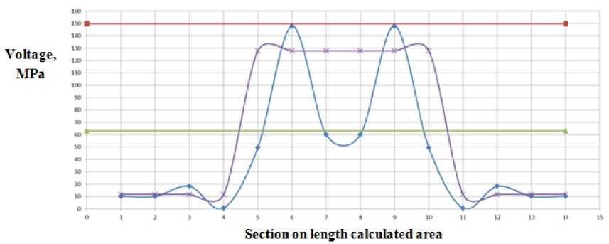
Fig. 6. Graph of stress distribution compensator number 3 in radius of three tap pipe outer diameters
Allowable compensation voltage was determined in all cases [8].
Below are graphs of the stress distribution on calculated cross sections of these models U-shaped compensators.
If you pay attention, you can see that the maximum voltage with and without consideration of coefficients are comparable in the first two computational models within approximately tap equal to three outer diameters of pipe. For the third calculation model similar graph is as follows
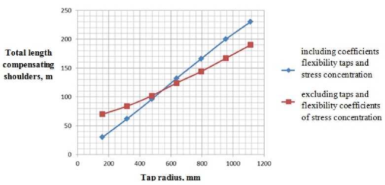
Fig. 7. A plot of the maximum total departure adjacent compensated shoulders the radius of taps curvature for calculation model compensator number 1
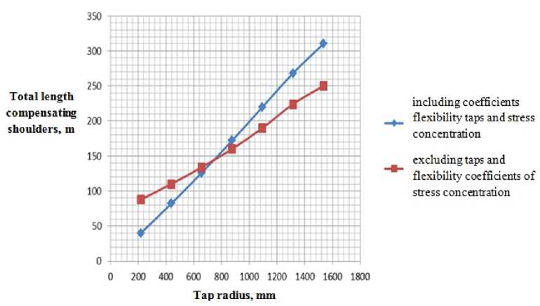
Fig. 8. A plot of the maximum total departure adjacent compensated shoulders the radius of taps curvature for calculation model compensator number 2
It is evident that a similar comparison with the first model calculations on the graph above is not observed. Now pay attention to plots of the maximum total departure from adjacent compensated shoulder radius of curvature taps.
These are graphs the first two computational models for compensators. It is seen that lines on graphs in both cases intersect at about 3.5 diameters (note markers on charts). Here is a chart of the third calculation model
Intersection happens here at 4 diameters. Therefore there is a lack of comparability graphs of stress distribution on cross sections of area.
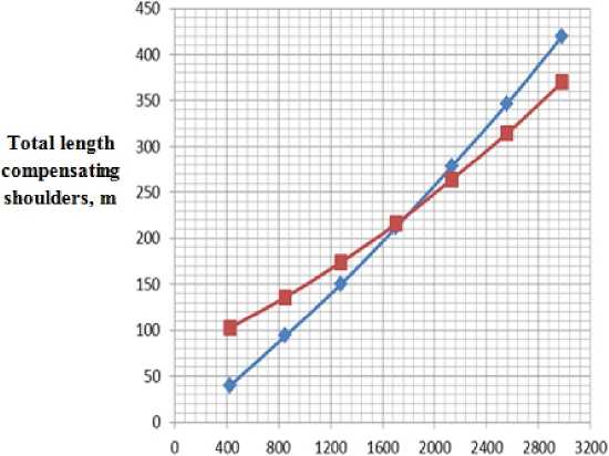
Tap radius, mm
including coefficients flexibility taps and stress concentration excluding taps and flexibility coefficients of stress cone:en trail on
Fig. 9. A plot of the maximum total departure adjacent compensated shoulders the radius of taps curvature for calculation model compensator number 3
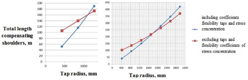
Fig. 10. Plots of the maximum total departure adjacent compensated shoulders the radius of taps curvature for calculation model compensator number 3 with a thickness of 12 mm (left) and 7 mm (right)
If the third calculation model to increase the wall thickness from 7 to 12 mm, the point of intersection graphs of maximum total departure from adjacent compensated shoulder radius of curvature taps shifts to the origin
Findings
Chart analysis suggests the following conclusions:
-
1. Most unfavorable from the viewpoint of safety factors is the use of taps in which the radius of curvature is one outside diameter of pipe
-
2. Increasing the radius of curvature taps from one to two outer diameters increases the maximum departure compensated shoulders twice.
-
3. In calculations coefficients of flexibility taps and stress concentrations should take into account because ignoring the latter leads to incorrect results.
-
4. In case of tap radius reduction and increasing the wall thickness of pipe in calculation model there is comparing the coefficients of flexibility and taps them stress concentration to unity.
