The Intensity-Curvature Functional of The Trivariate Cubic Lagrange Interpolation Formula

Published Online August 2013 in MECS (http://www.

The Intensity-Curvature Functional has been invented while describing a novel approach to improve the approximation properties of the bivariate linear interpolation function [1] and has been recently studied while reporting qualitative results obtained with Magnetic Resonance Imaging [2]. The idea to measure the signal-image intensity-curvature content is novel in literature. In this works the measurement of the intensity-curvature content is performed when the signal-image has been fitted with a math formula in order to perform the signal processing technique called interpolation [3-5]. Within the context of the measurement of the signal-image content, interpolation assumes the role of providing the Intensity-Curvature Functional [6-7] with both of the model function and the intra-pixel re-sampling location. The intra-pixel resampling location is necessary in order to calculate both of the signal and the second order partial derivatives of the interpolation formula (model function).

The benefits of the Intensity-Curvature Functional have been extensively explored within the domain of the improvement of the approximation characteristics of the mathematical functions [6-7]. It is yet to be ascertained the benefit of the Intensity-Curvature Functional in terms of its capability to re-image the signal. The concept of re-imaging the signal consists in creating a novel map of the signal which highlights characteristics of the signal-image likewise discernible in the original form and portrait such characteristics under a different perspective. For example, this manuscript presents Intensity-Curvature Functional images which emphasizes on the intensity-curvature content of human brain structures such as the sulci (see Fig. 6 and Fig. 7 in the results section). Thus, the imaging modality chosen in this work to approach the study of the qualitative characteristics of the Intensity-Curvature Functional is the Magnetic Resonance Imaging (MRI) of the human brain. And, the interpolation formulae chosen to illustrate the results are the trivariate and bivariate cubic Lagrange formulae [7]. As reported earlier [2] the Intensity-Curvature Functional is a dimensionless quantity because it is a ratio between terms of the same nature: the multiplication between the signal-image intensity and the sum of second order partial derivatives of the interpolation function. The signal-image mapping through the Intensity-Curvature Functional displays the characteristic of portraying under a different perspective the features of the original signal-image and this characteristic is correlated with the math formulation of the Intensity-Curvature Functional. Naturally, the joint information content of signal-image intensity with the sum of second order partial derivatives of the model function provides the Intensity-Curvature Functional with the math engineering necessary to measure the intensity-curvature content. And, the IntensityCurvature Functional can highlight features of the original signal-image, which are likewise discernible. In section II the theoretical background is given along with the formulation of the trivariate cubic Lagrange polynomial. In section III qualitative results obtained with MRI images of the human brain are presented. Section IV discusses the requirements for the calculation of the Intensity-Curvature Functional and the characteristics of the mapping derived through the measurement of the signal-image intensity-curvature content.

• II.    THEORY

The theoretical requirements of the model interpolation function were given in [2]. Formula (1) supersedes the (1) given in pg. 16 in [2] and it is the correct one to calculate the Intensity-Curvature Functional.

∆ E( x ) = { Σ ij ∫ f( 0 ) [ ∂ ²f( x ) / ∂ x i ∂ x j ] x = 0 d x } /

{ Σ ij ∫ f( x ) [ ∂ ²f( x ) / ∂ x i ∂ x j ] x = x d x } (1)

The derivatives included in the sums are all those partial second order derivatives of the Hessian of the model interpolation function. The model interpolation function chosen in this study is the trivariate (three dimensional) cubic Lagrange interpolation formula given in (2).

LGR 3 (x, y, z) = f (0, 0, 0) + ω ₁ ⋅ [ (1/2) (x + y + z)³ -(x + y + z)² - 1/2 (x + y + z) + 1 ] + ω ₂ ⋅ [ - (1/6) (x + y + z)³ + (x + y + z)² - (11/6) (x + y + z) + 1] (2)

The numerical values of the constants ω 1 and ω 2 are sums of the pixel intensity value in the neighborhood of the pixel to re-sample (f (0, 0, 0)) [7]. The intensitycurvature term before interpolation E₀(x, y, z) (which is the numerator of (1)) and the intensity-curvature term after interpolation E_I N (x, y, z) (which is the denominator of (1)) are given in (3) and in (4) respectively.

E₀(x, y, z) = { 9 ⋅ xyz ⋅ f(0, 0, 0) ⋅ [ - 2 ω ₁ + 2 ω ₂] } (3)

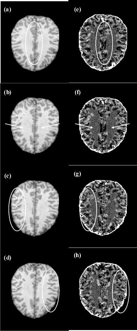
Figure 1. In (a), (b), (c) and (d) are shown four slices of an MRI volume in the proximity of the motor cortex, and in (e), (f), (g) and (h) are shown the corresponding IntensityCurvature Functional maps calculated with (1) when using the trivariate cubic Lagrange interpolation function to re-sample of the misplacement of 0.1mm along all of x , y and z axis respectively. The pixel matrix size is 182x218 with pixel size of 1.0mm x 1.0mm.

Where the values of П(1), П(2), П(3) and П(4) are given in (5), (6), (7) and (8) respectively.

E in (x, y, z) = { 9 • f(0,0,0) • { to i • [ 3 П ⁽¹⁾ - 2 xyz ] + to ₂ • [ - П ⁽¹⁾ + 2 xyz]} + 9 • {[ (3/2) to 1 ² - to 1 to ₂ + (1/6) to ₂²] • П ⁽⁴⁾ + [-4 to 1 ² + (16/3) to 1 to ₂ - (8/6) to ₂²] • П ⁽³⁾ + [ (1/2) to 1 ² - (54/6) to 1 to ₂ + (23/6) to ₂²] • П ⁽²⁾ + [ 4 _{Ю 1} ² + (28/6) _{Ю 1} to ₂ - (28/6) to ₂ 2 ] • П ⁽¹⁾ + [ - 2 _{Ю 1} ² + 2 to 2 ²] xyz} }                                    (4)

П⁽¹⁾ = (x²yz/2 + xy²z/2 + xyz²/2)                 (5)

П⁽²⁾ = (x³yz/3 + xy³z/3 + xyz³/3 + x²y²z/2 + x²yz²/2

+ xy²z²/2)                                   (6)

П⁽³⁾ = (x⁴yz/4 + x²y³z/6 + x²yz³/6 + x³y²z/3 + x³yz²/3 + x²y²z²/4 + x³y²z/6 + xy⁴z/4 + 2 3    23    222    32

zv y z 6 + x y z/3 + xyz + xyz 3 + x³yz²/6 + xy³z²/6 + xyz⁴/4 + x²y²z²/4 + x²yz³/3 + xy²z³/3)                          (7)

П⁽⁴⁾ = (x 5 yz/5 + x³y³z/9 + x³yz³/9 + x⁴y²z/4 + x⁴yz² /4 + x³y²z²/6 + xy⁵z/5 + x³y³z/9 + xy³z³/9 + x²y⁴z + x²y³z²/6 + xy⁴z²/4 + x³yz³/9 + xy³z³/9 + xyz⁵/5 + x²y²z³/6 + x²yz⁴/4 + xy²z⁴/4 + x⁴y²z/4 + x²y⁴z/4 + x²y²z³/6 + 4 x³y³z /9 + x³y²z²/3 + x²y³z²/3 + x⁴yz²/4 + x²y³z²/6 + x²yz⁴ x³y²z²/3 + 4 x³yz³/9 + 4 x²y²z³/12 +

22    42    24   232

zv y z 6 + xy z + xy z + xyz 3 +

4 x²y²z³/12 + 4 xy³z³/9)                   (8)

• III.    QUALITATIVE RESULTS

This section reports on the results of the calculation of the Intensity-Curvature Functional when re-sampling in three axial dimensions concurrently (Fig. 1 through Fig. 5) and also in two axial dimensions concurrently (Fig. 6 and Fig. 7). The images are MRI of the human brain and a contextual image.

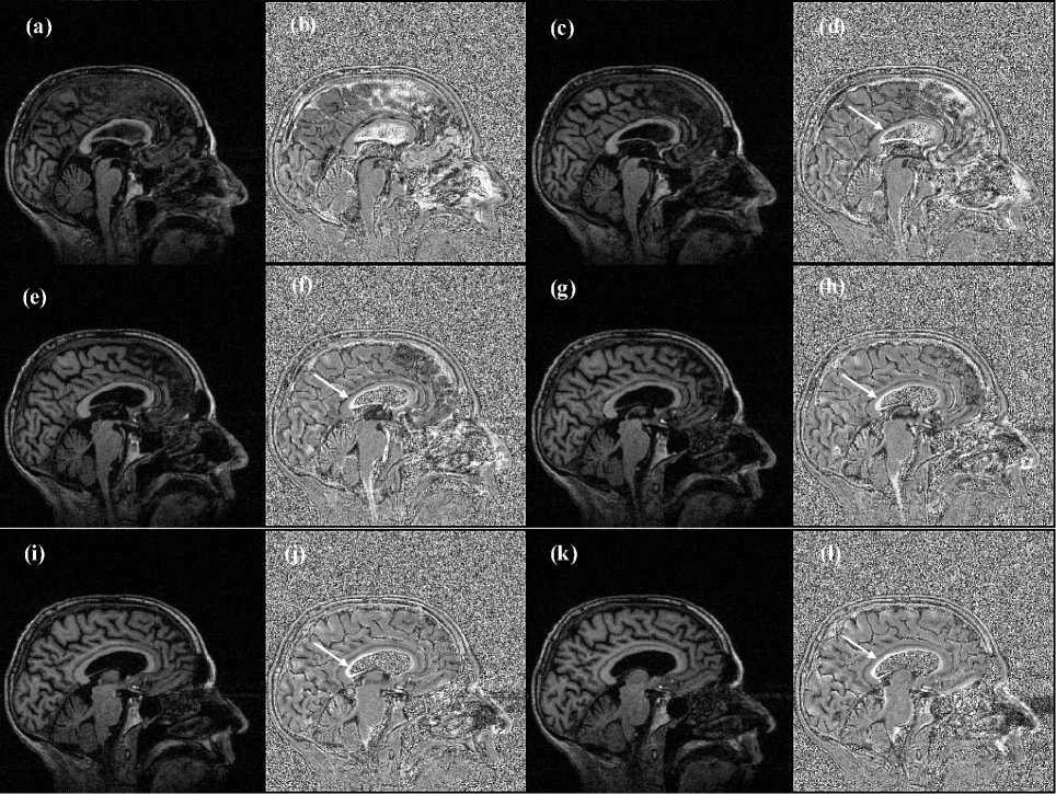
Figure 2. MRI of the human brain shown in (a), (c), (e), (g), (i) and (k) and the corresponding Intensity-Curvature Functional maps calculated while re-sampling with the trivariate cubic Lagrange interpolation function of the misplacement of 0.1mm along all of x , y and z axis concurrently are shown in (b), (d), (f), (h), (j) and (l). The pixel matrix size is 256x256 with pixel size of 1.0mm x 1.0mm.

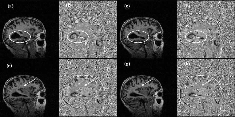
Figure 3. MRI of the human brain shown in (a), (c), (e) and (g). The Intensity-Curvature Functional maps are shown in (b), (d), (f) and (h). All of model function, misplacements, pixel matrix size and pixel size are the same as those of Fig. 3.

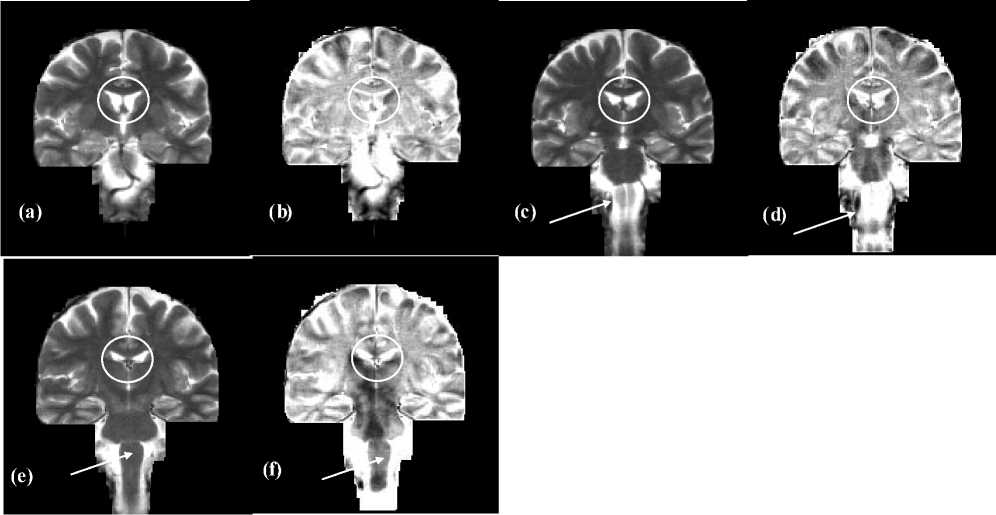
Figure 4. T2 Magnetic Resonance Imaging (MRI) three dimensional volume shown in (a), (c) and (e) (is Courtesy of: R. S.

Swenson, ~rswenson/Atlas), and the corresponding Intensity-Curvature Functional slice by slice shown in (b), (d) and (f). The pixel matrix size is 177x182 and the voxels ʼ size is 1.0 mm ×1.0 mm × 1.0 mm along the edges. The intensit-ycurvature functional images were calculated with the trivariate cubic Lagrange interpolation formula (2) when re-sampling of 0.1mm along all of x, y and z axis concurrently.

In Fig. 1.a the region of the brain enclosed in the white ellipse is mapped through the Intensity-Curvature Functional into Fig. 1.e. In Fig. 1.f is noticeable (see white arrows) the mapping of the white matter seen in Fig. 1.b. In Figs. 1.c, 1.d the region of the brain inside the white ellipse is mapped into the region of the brain seen inside the ellipses of Figs. 1.g and 1.h respectively. It is worth noting in Figs. 1.g and 1.h the portrait of the Intensity-Curvature Functional images of the sulci of the brain seen in Figs. 1.c and 1.d (see regions of the brain inside the white ellipses). More in general, Fig. 1 shows that the mapping of the Intensity-Curvature Functional is capable to keep the distinction between the white matter and the grey matter, and this is visible across the images with the increased gray level seen in the Intensity-Curvature Functional maps when compared with the brain images in (a), (b), (c) and (d). In Fig. 2 the MRI is shown along with the Intensity-Curvature

Functional maps. Specifically, the brain images seen in (a), (c), (e), (g), (i) and (k) correlates with the images (b), (d), (f), (h), (j) and (l) respectively.

The most visible feature of the Intensity-Curvature Functional maps is seen in (b), (d), (f), (h), (j) and (l) and consists of the portrait of the details of the human brain cortex along with the cerebellum and the spinal cord. Most visible is also (as pointed by the white arrows) the white contour located inside the ventricles. The MRI of Figs. 1, 2 and 3 belongs to the OASIS database: [8-13].

Fig. 3 shows four more slices of the brain volume seen in Fig. 2 along with the Intensity-Curvature Functional maps seen in Figs. 3.b, 3.d, 3.f and 3.h. The white circles in Figs. 3.a, 3.b, 3.c and 3.d enclose the ventricle of the brain: both in the MRI and in the Intensity-Curvature Functional; and highlight on the capability of the Intensity-Curvature Functional to portrait the features of the original signal-image from which it is calculated. The white arrows in Figs. 3.e, 3.f, 3.g and 3.h indicate the similarity between the MRI and the Intensity-Curvature Functional in the large extension of white matter of the brain.

Fig. 4 is relevant to T2 MRI images and shows the original data in (a), (c) and (e), and the IntensityCurvature Functional in (b), (d) and (f). The white circle in Fig. 4 hightlights on the similarity between the original MRI and the mapping seen in the IntensityCurvature Functional images, specifically when looking at the brain ventricles. The white arrows point to the similarity shown in the mapping of the spinal cord in Figs. 4.c, 4.d, 4.e and 4.f. For the remaining of the images in Fig. 4, the Intensity-Curvature Functional is quite effective in mapping both of the white and the grey matter of the brain.

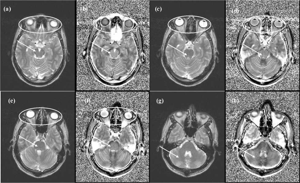
Figure 5. MRI of the human brain shown in (a), (c), (e) and (g) (courtesy of Casa di Cure Triolo-Zancla, Palermo - Italy) and the Intensity-Curvature Functional maps shown in (b), (d), (f) and (h). The model function fitted to the image data is the trivariate cubic Lagrange interpolation function (2). The misplacement employed to re-sample the images is 0.1 mm simultaneously along all of x, y and z axis of the coordinate system. The pixel matrix size is 256x256 and the voxels ʼ size is 1.0 mm × 1.0 mm × 1.0 mm along the edges. The images were cropped of 0.25" along the right and left edges to highlight the region of interest.

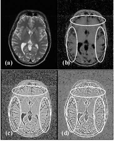
Figure 6. The MRI in (a) (courtesy of Casa di Cure Triolo-Zancla, Palermo – Italy) has been used to calculate the Intensity-Curvature Functional image maps seen in (b) (misplacement: (x, y) ≡ (0.5mm, 0.5mm), in (c) (misplacement:

(x, y) ≡ (0.7mm, 0.7mm) and in (d) (misplacement: (x, y) ≡ (0.9mm, 0.9mm). The images in (b), in (c) and in (d) show a high level of details (see inside the ellipses), emphasizing on the structure of the brain sulci. The images were cropped of 0.25" along the right and left edges to focus on the region of interest.

To investigate the aforementioned research question, the Intensity-Curvature Functional was calculated in two dimensions (on the basis of 2D images), and Fig. 6 and Fig. 7 provide illustrative results. The two dimensional cubic Lagrange interpolation formula (9) was used to calculate the Intensity-Curvature Functional of the images seen in Fig. 6.a and Fig. 7.a, and the IntensityCurvature Functional is shown in Figs. 6.b, 6.c, 6.d and Figs. 7.b, 7.c, 7.d respectively.

LGR₃(x, y) = f (0, 0) + α₃ ⋅ [ (1/2) (x + y)³ - (x + y)² - 1/2 (x + y) + 1 ] + α₂ ⋅ [ - (1/6) (x + y)³ + (x + y)² -(11/6) (x + y) + 1]                               (9)

The coefficints α 2 and α 3 of (9) are sums of the pixel intensity values in the neighbourhood of the pixel to resample f(0, 0).

Re-sampling was performed at the (x, y) intrapixel locations of: (0.5mm, 0.5mm) see Figs. 6.b and 7.b; (0.7mm, 0.7mm) see Figs. 6.c and 7.c; and (0.9mm, 0.9mm) see Figs. 6.d and 7.d. The images in Figs. 6.a and 7.a have 256x256 pixel matrix size with 1.00mm x 1.00mm pixel size. When looking inside the white ellipses in Figs. 6.b, 6.c and 6.d; it is possible to discern, specifically to the brain sulci, a pronounced level of details, and this behaviour is more visible in Figs. 6.c and 6.d than it is in Fig. 6.b. Similarly, Figs. 7.b, 7.c and

Fig. 5 is relevant to four slices of an MRI volume comprising of 26 slices. The trivariate cubic Lagrange interpolation formula (2) has been fitted to the data and the Intensity-Curvature Functional was calculated with (1) and (3) through (8), consistently with all of the 3D experimentations presented in this manuscript. The slices are presented in descending oder from (a) through (c), (e) and (g) and the corresponding IntensityCurvature Functional maps which are shown in (b), (d), (f) and (h) show strong correlation with the MRI, especially when looking at the eyes (see region inside the oval in Figs. 5.a, 5.b, 5.c, 5.d, 5.e and 5.f), and the brain structures shown by the white arrows in Figs. 5.a, 5.b, 5.c, 5.d, 5.e and 5.f. In Fig. 5.g and Fig. h emphasis is given to the capability of the the Intensity-Curvature Functional to portrait and highlight characteristics of the signal-image image specifically in the region of the cerebellum (as indicated by the white arrows), however as discernible in the rest of the images it is worth stressing on the non indifferent capabilities of (1) to highlight brain images details in all the regions of the cortical areas, when fitting the signal-image with the trivariate cubic Lagrange interpolation formula (2).

Another aspect which was investigated is the potentiality of the Intensity-Curvature Functional to provide benefits when re-imaging the signal. More specifically, the research question which was investigated tends to ascertain as to if it is possible to discern in the Intensity-Curvature Functional images, a level of details yet not highlighted as they appear in the original images.

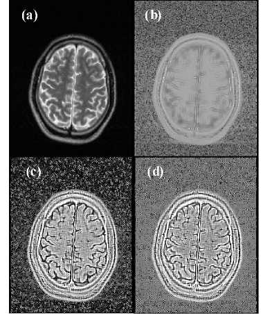
Figure 7. The MRI in (a) is courtesy of Casa di Cure Triolo-Zancla, Palermo – Italy, and it has been used to calculate the Intensity-Curvature Functional image maps seen in (b), (c) and (d). Re-sampling was performed with a misplacement of (x, y) ≡ (0.5mm, 0.5mm) in (b), with a misplacement of (x, y) ≡ (0.7mm, 0.7mm) in (c), and with a misplacement of (x, y) ≡ (0.9mm, 0.9mm) in (d). The images were cropped of 0.25" along the right and left edges to highlight the region of interest.

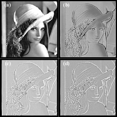
Figure 8. The original lena image is shown in (a) with a pixel matrix size of 232x232. The Intensity-Curvature Functional images obtained when re-sampling with (9) are shown in (b): misplacement (x, y) ≡ (0.5mm, 0.5 mm), in (c): misplacement (x, y) ≡ (0.7mm, 0.7 mm), and in (d): misplacement (x, y) ≡ (0.9mm, 0.9 mm).

7.d show the Intensity-Curvature Functional of the image shown in Fig. 7.a. The effect of the calculation of the Intensity-Curvature Functional consists once again in hightlighting the cortical structure with particular emphasis on the sulci of the motor cortex, with this aspect being more accentuated in Fig. 7.c and 7.d than in Fig. 7.b.

Overall, from Figs. 6.b, 6.c, 6.d, 7.b, 7.c and 7.d, it can be inferrred that the value of the intra-pixel location where re-sampling takes place is of relevance in hightlighting of the original image features of Fig. 6.a and Fig. 7.a. It is due to remark that the re-imaging process through the use of the Intensity-Curvature Functional is novel in literature as well is novel to reimage Magnetic Resonance Imaging data as shown in Figs. 1 through 7 of this manuscript.

To complete the presentation of the results, Fig. 8 shows the behavior of the Intensity-Curvature Functional for a contextual image. In Fig. 8.a is shown the original image, in Fig. 8.b, 8.c and 8.d are shown the Intensity-Curvature Functional maps when the misplacement used to re-sample the image with (9) is: (x, y) ≡ (0.5mm, 0.5mm) in Fig.8.b, (x, y) ≡ (0.7mm, 0.7mm) in Fig. 8.c, and (x, y) ≡ (0.9mm, 0.9mm) in Fig. 8.d. Fig. 8 confirms the findings reported when resampling the MRI images and therefore extends the domain of application of the Intensity-Curvature Functional to non MRI imaging.

• IV.    DISCUSSION AND CONCLUSION

A.    Requirements for the Calculation of the Intensity

Curvature Functional

To discuss these results it has to be clarified that the original intent of the Intensity-Curvature Functional was that one of the improvement of the approximation characteristics of the interpolation functions [1, 2, 6, 7]. While studying the improved interpolation paradigms it has become increasingly noticeable the fact that the Intensity-Curvature Functional shows the main characteristic in that of portraying and highlighting the signal-image feature from which it is calculated. The aforementioned characteristic of the Intensity-Curvature Functional is consequential to the use of the joint information content provided through the intensitycurvature measurement. Due to report that the intensitycurvature measure studied here can be calculated when the following three conditions are met.

One is that a model function (the interpolation function) is fitted to the signal-image. The second condition requires that the model function benefits of the property of second order differentiability, which is the property of existence of non null valued second order partial derivatives of the model function. The third requirement is that the signal-image is re-sampled at an intra-pixel (2D) or intra-voxel (3D) location.

Indeed, for the calculation of the numerator of (1) the signal-image is the original one as indicated by the notation f( 0 ) whereas the second order derivatives are calculated at the grid point of the pixel matrix either in 2D or in 3D. Whereas, for the calculation of the denominator of (1), the definition of Intensity-Curvature Functional given in (1) does require that both of the signal-image f( x ) and the sum of second order partial derivatives are calculated at the intra-pixel location x , either in two or three dimensions. Additionally, from (1) it is not acceptable that the second order partial derivatives are null because the ratio in (1) cannot admit null denominator.

B.    Characteristics of the Intensity-Curvature Functional

Another non indifferent characteristic of the IntensityCurvature Functional is that one of being a direct measure of the intensity-curvature content, which is a concept introduced in [2] along with other intensitycurvature measures and while studying the use of other interpolation functions.

Although a generalization to all of the model functions having the property of second order differentiability is possible [6, 7], the IntensityCurvature Functional studied in this manuscript is the one calculated in three dimensions with the trivariate cubic Lagrange interpolation function and in two dimensions with the bivariate cubic Lagrange interpolation function.

Results confirm the property of the IntensityCurvature Functional to be an intensity-curvature measure of non indifferent importance and this is demonstrated through the similarity with the signalimage and through the capability to portraying and highlighting, with high level of details, the features of the signal-image.

Additionally, the possibility to tune the re-imaging process through the change of the value of the intrapixel (2D) or intra-voxel location (3D), provides the Intensity-Curvature Functional with another feature, which is that of displaying the original image it derives from, placing the emphasis on specific or particular details of the original image. The aforementioned behavior might offer the possibility to re-image the signal placing the emphasis on the image details which are in need to be highlighted and thus may yield a novel imaging tool to be used to study biomedical images such for instance the Magnetic Resonance Imaging of the human brain. The domain of applicability of the Intensity-Curvature Functional can be extended also to other imaging modalities as suggested by the data presented in the results section.

• C.    Conclusion

In conclusion, the Intensity-Curvature Functional is a direct measure of the intensity-curvature content of the signal image. Experimentations with the trivariate cubic Lagrange interpolation function, which was used to resample the images, confirm the capability of the aforementioned measure to highlight and reproduce quite faithfully and generally the level of details of the signal-image. Experimentations with the bivariate cubic Lagrange interpolation function, used to re-sample the original image, instead, reveal the potentiality of the Intensity Curvature Functional to highlight particular and specific features of interest in the MRI brain images as well as in other imaging modalities.

ACKNOWLEDGMENT

Hereto publishing findings that benefit from OASIS data , we are due to mention the following grant numbers: P50 AG05681, P01 AG03991, R01 AG021910, P20 MH071616, U24 RR021382 . The author is very grateful to Professor Fadi P. Deek, New Jersey Institute of Technology, U.S.A., for the invaluable suggestions provided during the developmental efforts of this research. Formulae (2) through (9) and figures 4.a, 4.c, 4.e, 5.a, 5.c, 5.e, 5.g, 6.a and 7.a are reprinted with permission from [7].