The Mathematical Model for Research of the UAV Longitudinal Moving

Published Online October 2021 in MECS DOI: 10.5815/ijcnis.2021.05.03

Nowadays the majority of countries of the world emphatically work toward to equip national armed forces, other security and rescue State bodies, as well as civil sectors, by UAV of different functionality. They have very broad functional and size diapason: from nana - UAV, for example, "Black Hornet" (Prox Dynamics, Norway) with weight 16 grams and flight range approx. 30 minutes, to strategic UAV RQ-4 "Global Hawk" (Northrop Grumman, USA) with take-off mass 14,6 tons and flight range approx. 32 hours. Funding on UAV development and purchasing in the world constantly grows, as we can see from the 2013-2022 UAV market forecast [1,2], Table 1.

The sphere of the civil UAV usage is also increasing. Except such areas like monitoring highways, railways, pipelines, electric power-lines, meteorological and ecological monitoring, that became already traditional, the new directions of UAV using are being developed. Level of modern technologies, as well as the forecast of researches conducted by leading companies that develop UAV allows to speak about opportunity of broader UAV application. This, first of all, cargo and mail delivery, casualty’s evacuation, goods and medications transportation, crop processing, passenger’s transportation, etc.

It should be noted that it is typical trend today when UAV design and production technologies are exchanging from civil to military sphere and vice versa. Moreover, the first trend increases because civil UAV designers (producers) have not so much limitations as their military colleges.

That allows them produce less expensive UAV using а more wide range of components and software, such as communication systems and transmitting protocols, digital maps, digital sensors, engines and energy sources.

Thereby, one can see, that urgency of studying UAV development issues is confirmed not only by real examples of their efficient application, but also by estimation specialist in perspective of UAV further development.

Table 1. Market UAV on 2013-2022

UAV class	The cost, billions $	% $
Tactical	15.94	40.7
MALE	13.56	34.6
HALE/UCAV	8.39	21.4
Man Portable	0.664	1.7
Civil	0.638	1.6

UAV creation, regardless of their application sphere and functionality, expects the development of appropriate control systems. It is important that for any selected type of the UAV control system [2] syntheses of this control system first of all demands developing the mathematical model of the object of control which will fits the process in question adequately. An operation of UAV during the completion of a task is a complex process requiring comprehensive technical means and systems. The control system of UAV is one of the most important systems. Its task is to measure, evaluate, and control flight parameters, as well as properly control the flight and observation systems. Thanks to the use of complex microprocessor systems, the comprehensive automation of the mentioned processes is possible.

Thus, this paper studies the questions of developing and justification of the adequate aerodynamic mathematical model on given aerodynamic, geometric, mass and inertial data of the longitudinal moving the perspective high-altitude long-endurance UAV.

As object of the research, shall choose hypothetical high-altitude and long-range perspective UAV, for example, the type "Altair" (Fig. 1). The input data for calculation mathematical model coefficients for longitudinal motion of perspective UAV (hereinafter - a UAV model) are presented in the Table 2.

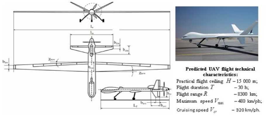
Fig.1. Shema UAV for calculation with predicted flight technical characteristics

Table 2. The input data for calculation of coefficients of the mathematical model

Parameter	Value	Parameter	Value
Take of mass m , kg	4760	Root chord of horizontal tail bOht, m	1.2
Wing aria Sw, m2	26.8	End chord of horizontal tail bkht, m	0.6
Under the fuselage wing area S wF , m2	1.91	Relative root of horizontal tail A h t	6.47
Wing span l w , m	20	Aria of vertical tail Sv t , m2	4.38
Wing Root chord bOw , m	1.95	Height of vertical tail hv t , m	1.3
Wing End chord bk , m	0.73	Root chord of vertical tail bOu , m	1.4
Sweep angle along the leading edge of the wing % ^w, deg	2.0	End chord of vertical tail bkv , m	0.7
Constriction of wing T]w	2.67	Relative root of vertical tail Av t	1.54
Middle of chord of wing baw , m	1.43	Elevators length le , m	5.4
Relative root of wing A w	14.93	Width of elevator h e , m	0.25
Relative coordinate center of mass, xT	0.31	Aria of elevator    S e , m2	1.35
Length between center of mass and ¼ middle of chord lcmch , m	3.4	Relative root of elevator A e	21.6
Relative coordinate of focus X f	0.36	Aria of middle section of fuselage Sm F , m2	0.75
Aria of horizontal tail S h t , m2	5.24	Fuselage length LF, m	11
Swing of horizontal tail l h t, m	5.82	Relative root of fuselage A f	8.4

2. Coefficients Calculation for The Model

Calculation aerodynamic characteristics are executed in accordance with formulas from [3, 4]. The coefficient of the drag under zero elevating force

e     aa x     xxw Sw   SWJ where k = 1.05...1.1 - the coefficient, taking into account our ignorance;

C_xw = C_xp(1 — kiS_wF/S_w) + ЕДС_Х the drag coefficient of the wing;

C_xF = C_xpF + ДС_хР - the drag coefficient of the fuselage;

Cxi = C_xaS_m/S_w - the drag coefficient of the landing gear of the UAV.

In accordance with [3]:

value of the drag coefficient of the profile of the wing is about Cxp = 0.0092;

the factor, taking into account interference between wing and fuselage ki = 0.5 ;

the factor of the drag coefficient of the wing, taking into account irregularities of the wing, presence of the slots between wing and its mechanization SA C _x = 0.002 ;

the factor of profile resistance of fuselage C_xpF = 0.071;

the additional coefficient of resistance, taking into account the form and irregularities of fuselage A C_xF = 0.02;

the factor of the drag coefficient of the landing gear UAV C_XQ • S_mF = 0.086 .

By substituting the accepted values of the coefficients and the source data from the Table1 2 to the formula (1), we’ll get the following result

Derivative from the coefficient of lifting power on angle of the attack whole UAV calculated by the formula (2)

I ^f-yf^(1—'^HQ-^    ^c “f ^s m

Sw        Sw

pT'+z - the derivative from coefficient of lifting power on angle of the attack of wing;

Here V yw p =    1—

2 \cosz1

1              2

+ "cosx ) + A (p+i) - the ratio of the wing perimeter to its span,

/ 1 - leading edge and / 2 trailing edge of wing;

С _t = 0'085^ ^{6 1} - the derivative from coefficient of lifting power of horizontal tail on angle of the attack of horizontal tail;

c“ ea = 46.2 y— kxkyk,]kz- the derivative from the angle of slant flow from the angle of attack UAV, were

kx = 1.55 -0.85(2lht/lw) + 0.3(2lht/lw)2;

ky = 1- 1.7(2 - 2yht/l^)2yht/lw;

Substituting the accepted value of the braking coefficient of flow in the field of the horizontal tail: k h _t = 0.9 with derivative from coefficient of lifting power of fuselage on angle of the attack of UAV: C “ _F = 0.035 and the source data of the Table 2 in the formula (2), we’ll get the following result

Coefficient mWz = -0.69a h t"L htAht                                            (3)

here a _{h t} =

^A h t = ⁵ h t ^ h t , ё _ ^ h t

^{5 h t} = b_aw , T _ ^Lht ^L h t = ,  .

t w

Substituting the accepted initial data in Table 2 to the formula (3), we’ll get the following result

Coefficient

Substituting the initial data in Table 2 and numeric value of the derivative C ? to the formula (4), we’ll get the following result

The coefficient of effective of elevator mze = -khtAhtah tne ht180 к

here n e h t =

Substituting the initial data in Table 2 and numeric values of coefficients to the formula (5), we’ll get the following result:q

The results of the calculation of the coefficients of aerodynamic forces and moments of UAV (Table 3)

Table 3. The results of the calculation UAV coefficients of aerodynamic forces and moments

С x	C;	m ^z	m ?	5e mz e
0.016	5.018	-4.863	-0.251	-0.7

Shot-period longitudinal move-UAV with sufficient accuracy reflects the linear model [5, 8]:

Дшг + am Да + а“гДа)2 = а^ Д6е                              (6)

'4Z            ''z              ''z    “

ДУ = шгД9 = Д9 + Да.

Here

- ( mV ) ^{- 1}

аа mz

z

■ ( I z ) ^{- 1}

— ( I z ) ^{- 1}

a ^m m_z

■ ( I z ) ^{- 1}

Substituting next equation

Y = C^aqSw,           Mz = m“aqSwbaw,

MZZ = m“ZtozqSwbaw,   M8ze = m5ze 3eqSwbaW,

pV2 q = —, to the formula (7) and taking into account that m“Z = mzzt^-, we’ll get the following equation for calculation coefficients of model (6), which were expressed through aerodynamic forces and moments UAV from the Table 3

a “ =- ( mV ) ^{- 1} ( C ^ qS w ) , a ^a™. =— ( I _z ) — 1 ( m^S w b _a ) , a m z =- ( I z )^{- 1} ( m T qS w b a ) , a m , =— ( I z ) — 1 ( m f e qS w b a ) .

To calculate coefficients in the (8) the inertia moment should be defined. According to the [6] we’ll calculate the inertia moment using the following estimate formula

Iz = izmL2Fp

After calculation we’ll get the following result

Iz = 17278.8kg ■ m2.

So, we’ve got all the initial data and analytical expressions for calculating coefficients of UAV model.

Calculations of UAV model coefficients for different speeds and flight altitudes were performed by the MathCAD package. The results of the calculations are presented in Table 4.

Table 4. The UAV model coefficients for the different speeds and flight altitudes

H , m	V , kmph	α a y , s–1	α a mz , s–2	ω z a mz , s–1	S. a k t z . s-2	7 So ka		toa > s–1	S a	Т θ , s	Flight mode
0	25	–1,22	1,67	0,66	–4,59	1,86	2,26	1,57	0,60	0,82	RI
1000	27	–1,19	1,77	0,65	–4,86	1,92	2,29	1,59	0,58	0,84	RII
	35	–1,55	2,97	0,84	–8,17	1,92	2,96	2,07	0,58	0,65	RIII
5000	28	–0,82	1,26	0,44	–3,46	2,13	1,75	1,27	0,50	1,22	RIV
	44	–1,29	3,11	0,70	–8,55	2,13	2,75	2,00	0,50	0,78	RV
7500	31	–0,69	1,17	0,37	–3,21	2,26	1,55	1,19	0,44	1,46	RVI
	46	–1,02	2,57	0,55	–7,06	2,26	2,30	1,77	0,44	0,98	RVII
13000	32	–0,34	0,59	0,18	–1,63	2,49	0,84	0,81	0,32	2,96	RVIII
	48	–0,517	1,33	0,27	–3,67	2,49	1,26	1,21	0,32	1,97	RIX
15000	35	–0,27	0,52	0,15	–1,42	2,556	0,69	0,75	0,28	3,71	RX
	48	–0,37	0,97	0,2	–2,68	2,56	0,95	1,02	0,28	2,70	RXI

Further studies of the model were performed using the apparatus of transfer functions, which are obtained by applying the Laplace transform of equations (6):

Software package MathLAB was applied while conducting researches of the UAV model.

The study of the UAV model was conducted by the following sequence: adequacy estimation, estimation of dynamic characteristics for the longitudinal controllability, analysis of temporary characteristics and analysis of logarithmic frequency characteristics.

V.V (P)   k..(10)

wS(p) = k^,(11)

^k 2 ^k 4

^5(p)=kTk3,

z

W8=(p) = ^-.(13)

^k 2 ^k 4

Here ко = k^^ki = к5ме2ш;2,к2 = p2 + 2^aP + ^.Лз = Te(p + 1),^ = p> where

л 5= к Se = k a        ^ 2’	Se , S e _ k a kM z    T T e
to a = ^^ ^z - ^ mz ^ y > ^ ^	л ^z_na _ amz - g y    _ “  2^a >  e ~    a“'

• 3.    Adequacy Estimation of the UAV Model

• 4.    The Estimation of Dynamic Characteristics for the Longitudinal Controllability of the UAV Model

• 5.    Analysis of Temporary Characteristics of the UAV Model

It is known that model of the UAV longitudinal motion is defined by three parameters: frequency of own shortperiod oscillation to_a , damping decrement f_a, time constant, which characterizes the maneuverability of UAV during its longitudinal motion Т g . Analysis of these parameters, given in Table 4, showed that they adequately characterize longitudal UAV motion when the flight modes change. The UAV model adequacy is confirmed by the following: with decreasing the flight velocity and increasing the flight height – the frequency of own short-period oscillation decreases from 1.572 s^-1 to 1.023 s^-1; with increasing the flight height – the damping decrement decreases from 0.597 to 0.278, at the same time the time constant increases from 0.821 s to 2.704 s; with increasing the flight velocity the time constant is decreases.

The estimation of dynamic characteristics of the UAV model allows to draw the following conclusions: range of the change of variation of the decrement damping (with the exception of the flight mode RX, RXI) is found within acceptable area of controllability f_a = 0.35.1.2 [7,8,9]. Diapasons of the change the frequency own short-periodic fluctuations for all flight modes of UAV is found outside the area of acceptable controllability ш_а =2...5 s^-1 [7]. These conditions need the automatic system of control (ASC) for improvement of the characteristics to stability and controllability UAV.

Temporary characteristics of model UAV (described by system of linear differential equations, presented in operator form) are identified, as reactions of models to standard impacts (in this case reaction to stepped function). Reactions of the UAV model to such impact are called the transition functions [10].

These transition functions are presented on Fig. 2 and Fig. 3. The transfer functions of the UAV model and their graphs for the RVI flight mode (V=310 km/ph, H=7500 m) are presented on Fig. 4.

The qualitative analysis of transition functions graphs of the UAV model testifies that these graphs adequately reflects the processes of changing parameters of the UAV short-periodic longitudal motion.

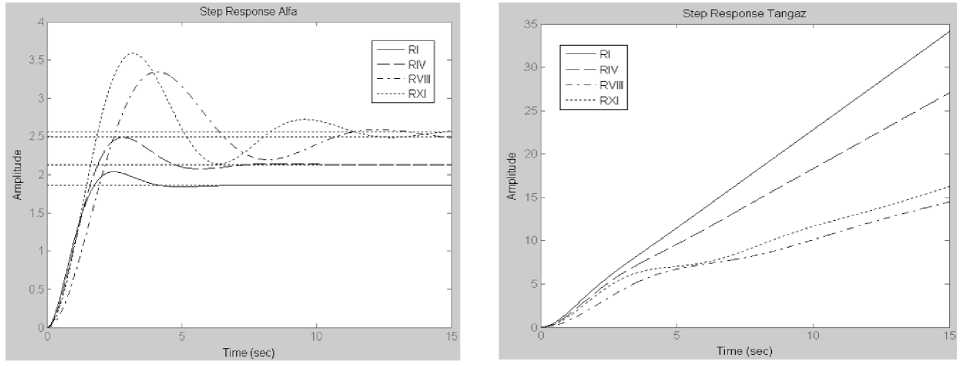
Fig.2. Transition functions of UAV model by angles of attack and pitch for different flight modes

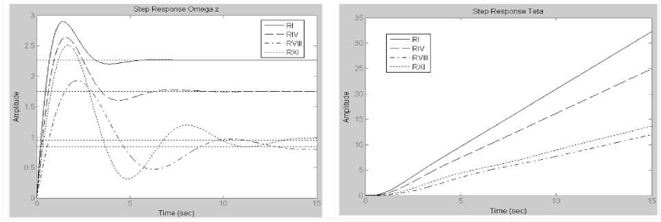
Fig.3. Transition functions of model UAV by angular speed of the pitch and the angle of tilt the trajectory for different flight modes

So, transition function graphs of such parameters as the angle of attack and the pitch angular speed have a pronounced oscillatory nature. The transition function graph of the tilt angle of trajectory seeks to linearly change in time. Similar picture with small fluctuations is observed for separate modes for the pitch angle.

The quantitative estimation of transition processes for the attack angle and the pitch angular speed is shown in the Table 5. Regulation time and overregulation time are the most important criteria of the quality of transition processes.

Table 5. Quantitative estimation temporary logarithmic and frequency characteristics of UAV model

Flight mode	Temporary characteristics				logarithmic frequency characteristics
	Regulation time t p , s		Overregulation time Δ h m , %		Amplitude stability margin Δ L , Db	Phase stability margin Δφ, deg.
	δ В W α	δ В W ω z	W δα В	δ В W δω Вz	δ В W θ	δ В W α	δ В W ω z	δ В W ϑ	δ В W θ
RI	3,78	4,46	9,65	27,93	–1,62	61,8	99,3	28,8	–8,41
RIV	6,37	5,83	16,62	50,48	–2,83	46,8	98,5	22,9	–16,1
RVI	7,01	8,3	21,03	67,18	–3,31	40,4	97,8	20,2	–19,9
RVIII	13,79	15,98	34,04	128,07	–4,17	27,6	–160 98,3	14,1	–28,6
RXI	13,53	15,22	39,94	163,06	–4,41	23,4	–166 95,1	12,1	–31,9

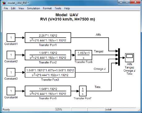
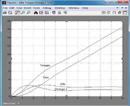
Fig.4. The transfer functions and graphs transition functions of the UAV model in MathLAB for flight mode RVI (V=310 kmph, Н=7500 m)

The estimation of the regulation time was conducted under condition that for the well damped UAV model (0.5 < fa < 1) this time is inversely proportional to own frequency of non-damping vibrations. Only mode RI for the angle of attack transfer function corresponds to this condition.

The overregulation estimation for the angle of attack of the transfer functions is evidence of the fact that for RI and RIV modes the overregulation is no more than 20 % (limit value). In other modes, it exceeds this limit value (20 %), wherein, for the pitch angular speed transition function it exceeds more than 8 times.

• 6.    Analysis of Logarithmic Frequency Characteristics of the UAV Model

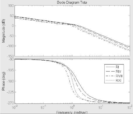
Logarithmic frequency characteristics (LFCH) of UAV models give us an idea of the UAV ability to monitor the deflection of longitudinal control loop elements. Also LFCH serves the source for designing and studies of UAV control systems. On Fig. 5 and Fig. 6. LFCH, corresponding to transfer functions W^^e(p), Wy^e(p), W^ ® (p), W^^e(p) from (5) – (8) and presented.

The logarithmic amplitude frequency (LAFCH) and phase frequency characteristics’ (PHFCH), shown on Fig. 5 and Fig. 6. They define the dependency of the amplitude and phase of the fluctuations angles of attack and pitch, angular speed of the pitch and the angle of tilt the trajectory angular speed of the pitch and the angle of tilt from frequency.

The qualitative analysis of these characteristics shows that they match:

for the angle of the attack - the characteristics of the oscillatory link;

for the angle of pitch - series connection of oscillatory, forcing and integrating links;

for the angular velocity – series connection of oscillatory and forcing links;

for the tilt angle of the trajectory - series connection of oscillatory and integrating links.

The quantitative estimation LACHH UAV model is presented in Table 5.

Table 5 data analysis gives an idea of significant margin of stability on phase (Дф > 30⁰) for angle of the attack in the area of RI, RIV, RVI modes. For all that, for others flight modes, as well as for angle of pitch transition function the stability margin on phase is insufficient to provide control with acceptable characteristics. The margin of amplitude stability for transfer functions for the UAV model on the trajectory angle of tilt does not satisfy the condition Д1 > 6 Db

The Estimation of the dynamic characteristics of longitudinal controllability, temporal and logarithmic frequency characteristics of the UAV model gives an idea that aerodynamic characteristics of perspective high-altitude and long-flight-range UAV provide acceptable stability and control characteristics in a narrow ranges of flight modes (only for RI and RIV modes). In order to improve these characteristics for rest flight modes the introduction of automation devices to the UAV control system is required.

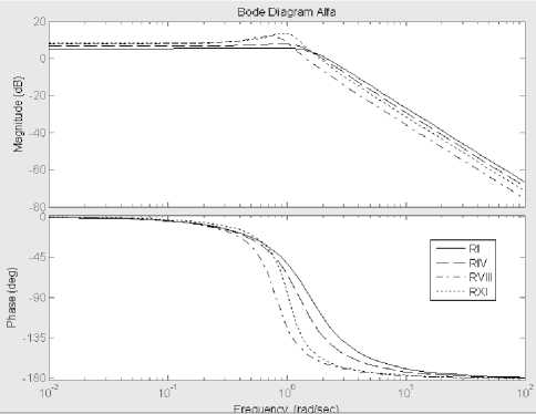
Fig.5. Logarithmic frequency characteristics’ (LFCH) to UAV model by angles of attack and pitch for different flight modes

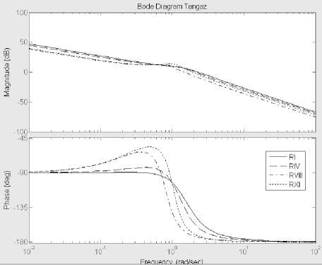
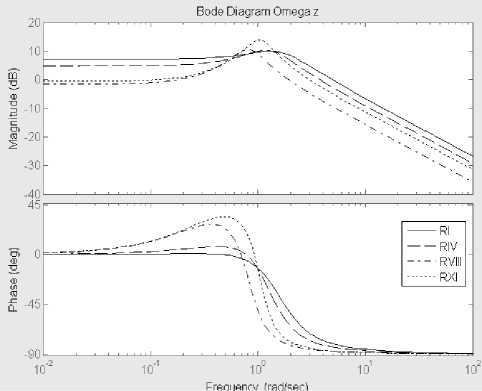
Fig.6. Logarithmic frequency characteristics’ (LFCH) to UAV model by angular speed of the pitch and the angle of tilt the trajectory for different flight modes

• 7.    Conclusion

The paper describes the mathematical model of perspective high-altitude and long-flight-range UAV. This model is obtained by calculations based on initial UAV geometric and mass data and also on aerodynamic forces and moments, with further transition from these characteristics to the calculation of coefficients of linear mathematic model for shotperiod longitudinal UAV motion.

The coefficients were calculated for 11 flight modes. Wherein, for 5 typical modes the analysis of temporary and logarithmic frequency characteristics, preliminary estimation of UAV dynamic characteristics, as well as adequacy mathematical model confirmation was conducted. The considerations presented in this paper will allow us to conduct the research in this field, namely UAV.

The UAV mathematical model, that was considered in the paper, can be used in the flight dynamics study, for synthesis of automatic control systems laws and for the other issues solution.

Conflict of Interests

The authors declare that there is no conflict of interests regarding the publication of this paper.