The method of equivalent strength conditions in calculating composite structures with a regular structure using multigrid finite elements

Author: Matveev А. D.
Journal: Siberian Aerospace Journal @vestnik-sibsau-en
Section: Informatics, computer technology and management
Article in issue: 4 vol.20, 2019.
Free access
Plates, beams and shells with non-uniform and micro-inhomogeneities regular structure are widely used in aviation and rocket and space technology. At the preliminary design stage, it is initially important to know whether the design safety factor meets the specified strength conditions. To determine the margin factor, it is necessary to solve the elasticity problem for the designed structure by the finite element method (FEM), taking into account its inhomogeneous structure, which requires large computer resources. In this paper, we propose a method of equivalent strength conditions (MESC) for calculating the static strength of elastic structures with a inhomogeneous regular structure. The proposed method is reduced to the calculation of the strength of isotropic homogeneous bodies using equivalent strength conditions. The MESC is based on the following statement. For any composite body V0 , there exists such an isotropic homogeneous body Vb and such a number p (equivalence coefficient) that if the body Vb stock coefficient satisfies 0 nb the equivalent strength conditions 0 pn1 nb pn2 , then the body V0 stock coefficient satisfies n0 the given strength conditions n1 n0 n2 , and Vice versa, n1 , n2 – given, the coefficients 0 nb , n0 , meet the exact solutions of elasticity problems constructed for bodies V0 , Vb . The method under consideration is reduced to FEM strength calculation of isotropic homogeneous bodies, which is the easiest to implement and requires less computer memory than a similar calculation of composite bodies taking into account their inhomogeneous structure. The procedure for determining the equivalence coefficients for a number of composite plates, beams and shells of rotation is described. High-precision multigrid finite elements generating discrete models of small dimension and solutions with small error are used in the construction of elastic solutions according to FEM for isotropic homogeneous bodies. The adjusted equivalent strength conditions are of the form pn1(11) nb pn2 (12 ) , where nb is the body Vb reserve coefficient and the values 1 , 2 correspond to the approximate solution constructed for the body Vb . Implementation of FEM for multigrid discrete models requires several 103-106 times less computer memory than for basic models. The calculation of the strength of a beam with a micro-homogeneous regular structure with the help of MESC is given.
Elasticity, composites, equivalent strength conditions, multigrid finite elements, plates, beams, shells.
Short address: https://sciup.org/148321703
IDR: 148321703 | UDC: 539.3 | DOI: 10.31772/2587-6066-2019-20-4-423-435
Text of the scientific article The method of equivalent strength conditions in calculating composite structures with a regular structure using multigrid finite elements
Introduction. The calculation of structural strength is one of the most important at the stage of a schematic design [1], which represents the technical and economic assessment of a design project. As a rule, structural strength calculation is performed according to margins of safety [1-3]. Accord- ing to the calculation, for the safety factor n of the designed structure V , the specified strength conditions have the following form n1 ^ n 0 ^ n 2, (1)
where n , n2 are given, n > 1.
At the stage of schematic design, it is primarily important for the designer to know whether the safety factor n of the designed structure V satisfies the specified strength conditions or not (1).
If the safety factor n satisfies the specified strength conditions, it is considered that the structure V does not fracture under given operational conditions. It should be noted that in this case it is not necessary to examine in detail the stress-strain state of the structure V . The calculation of the strength of the structure V reduces to finding its safety factor n and to the strength test (1) for the factor n 0 . The safety factor n 0 is defined according to the formula n 0 = < т г / < г 0 [1-3], where стг -limit stress of the structure Vo (yield stress [3]), < r0 - maximum equivalent stress of the structure V . It should be noted that the safety factor n corresponds to the exact solution of the elasticity problem formulated for the structure. If the maximum equivalent structural stresses are determined approximately, in this case the corrected strength conditions are used [4]. In the analysis of the stress-strain state of composite structures, the finite element method (FEM) is widely used [5-8]. The basic discrete models of structures with an inhomogeneous and microinhomogeneous structure, which consist of the first-order finite element (FE) and take into account their structures within the framework of the microapproach [9], have a very high dimension, which creates difficulties in the implementation of FEM on a computer. For such models, the multigrid finite element method (MFEM) [10–12] is effectively used, in which the multigrid finite element is used [13, 14]. It should be noted that FEM is a special case of multigrid finite element method, and if in solving boundary value problems in FEM multigrid finite elements are used, in this case, multigrid finite element method is implemented.
For practice, it is important to know the error of approximate solution that is used in the calculations. The error of approximate solutions can be estimated when they differ insignificantly from each other and at the same time form a sequence of solutions that quickly converges to the exact solution. When constructing such sequences, the splitting of the initial partition of the body area into FEs is applied. The splitting procedures used for partitions, which are built for a heterogeneous and microinhomogeneous (fibrous) structure, are complex and difficult to implement. Since the fibers have a small thickness, splitting of such partitions leads to a dramatic increase in the dimensions of discrete models. The implementation of FEM for such models requires large computer resources. In addition, certain restrictions are imposed on the law of splitting, due to the fact that at each step of splitting the partitions, it is necessary to take into account the microinhomogeneous structure by microapproach. As known, the splitting procedure used for discrete models of homogeneous isotropic bodies is the simplest to implement and requires less computer memory than for the bodies with an inhomogeneous and micro-inhomogeneous structure (taking into account their structure).
In this paper, the method of equivalent strength conditions is proposed for the static strength analysis of a linearly elastic structure V 0 with a heterogeneous (microinhomogeneous) regular structure consisting of plastic materials. For simplicity, we believe that the body V 0 has a fibrous structure. It is shown that the strength calculation of the composite body V 0 is reduced to the strength calculation (using FEM) of the isotropic homogeneous body Vb . The bodies V 0 , Vb have the same shape, size, fastening and loading. The elasticity moduli of the body V b and the fiber coincide. In the calculations, adjusted equivalent strength conditions of the form are used.
Pn 1(1 + ^ 1 ) ^ n b ^ Pn 2(1 - ^ 2 ), (2)
where £ 1 = 1/(1 - 5 p ) - 1, £ 2 = 1 - 1/(1 + 5 p ), p - equivalence number, nb - safety factor of the body Vb , nb = t r r / ^ b , сут - yield stress of the fiber, ob - maximum equivalent stress of the body Vb (being determined with the help of FEM), 5 p - error for the stress ob , 0 < 5 p < 1.
It is shown that if the safety factor
n
of the isotropic homogeneous body
Vb
satisfies the adjusted equivalent strength conditions (2), the safety factor
n
of the composite body
V
(corresponding to the exact solution to the elasticity problem) satisfies the given strength conditions (1). Thus, the implementation of the proposed method is reduced to constructing the adjusted equivalent strength conditions (2) and finding the safety factor
n
of the body
Vb
, i. e., determining the equivalence coefficient
p
and finding the maximum equivalent stress
ob
for the body
Vb
using FEM (with the error
5
p
). The equivalence coefficient
p
is found using the formula
p
=
cr0 / r
r
b
, where
The advantages of the method of equivalent strength conditions are the following. In the calculations, we use isotropic homogeneous structures that have the same shapes and sizes, fastening and loading, as composite structures. When analyzing the strain-stress state of isotropic homogeneous structures according to FEM, multigrid finite elements are used, which allow us to construct sequences of solutions that are fast converging to exact ones. It allows to determine the error for the obtained approximate solutions. Multigrid finite elements for isotropic homogeneous structures generate discrete models of small dimension and approximate solutions with a small error. The implementation of FEM for multigrid discrete models requires 10 3 ^ 10 6 times less computer memory than for basic ones. When implementing multigrid finite elements, splitting procedures for discrete models of composite structures are not used. An example of calculating the strength of a beam with a microinhomogeneous regular fibrous structure using multigrid finite elements is given.
Fundamental principles for the structures. The paper considers three-dimensional structures (bodies) for which the following conditions are satisfied.
Principle 1. Three-dimensional linearly elastic isotropic homogeneous and composite bodies (structures) are considered in Cartesian coordinate systems. These structures consist of ductile materials, have smooth boundaries, static loading, and the same operating conditions. Body loading functions are smooth functions. The bodies have boundaries that do not degenerate into points. The composite bodies consist of heterogeneous modules of isotropic homogeneous bodies, the connections between which are ideal, i.e., at the common boundaries of heterogeneous modules of homogeneous bodies, the functions of displacements and stresses are continuous. The displacements, deformations, and stresses of the multimodular bodies correspond to the Cauchy relations and the Hooke law of the three-dimensional linear problem of the theory of elasticity [15]. Equivalent stresses for elastic bodies are determined by the 4th theory of strength [1].
Equivalent strength conditions and equivalent structural strengths expressed in terms of safety factors. Let us suppose that two elastic structures V and V have the same shape, geometric dimensions, fastenings, and static loads, but differ in elastic moduli. Let the safety conditions be set for the safety factors n , n of the structures V , V respectively na < n1 < nb, (3)
n J < n 2 < n 2 , (4)
where n1, n2 > 1; n1, n2 , n1, n2 are given; the factor nx ( n2 ) corresponds to the exact solution of the elasticity problem posed for the structure V (V ).
Let us introduce the following definitions for the structures V , V .
Definition 1. If the fulfillment of conditions (4) for the factor n implies the fulfillment of conditions (3) for the factor n and vice versa: if the fulfillment of conditions (3) for the factor n implies the fulfillment of conditions (4) for the factor n , then the strength conditions (3), (4) will be called equivalent strength conditions, respectively, for the structures V , V .
Definition 2. Let the structures V , V , for which the conditions (3), (4) are equivalent strength conditions respectively, not be destroyed under the same operating conditions. Then we call the structures V , V equivalent in strength.
In practice, the strength equivalence of the structures V , V means that instead of the stressed structure V , the structure V can be used, and vice versa. It should be noted that, of the two structures equivalent in strength, it is appropriate to use a design that is more technological in manufacturing, meets specified technical requirements and requires less financial costs for manufacturing and operation.
The theorem on the existence of equivalent strength conditions. Let us consider the theorem that proves the existence of equivalent strength conditions for elastic composite structures (bodies).
Theorem 1. Let a predetermined static surface force q act on the three-dimensional linearly elastic composite body V (located in a Cartesian coordinate system Oxyz ), i.e., forces acting on the unsecured part of the boundary S q of the body V and volume forces p , where q = { qx , qy , qz } T , p = { px , py , pz } T : q x , q y , qz , px , py , pz - smooth function of the coordinates x , y , z .
At the boundary Su , the body V 0 is rigidly fixed, i.e., at S u : u = v = w = 0, S 0 = S u + Sq , S 0 -smooth boundary of the body V . The body V consists of V components, i.e., plastic, multimodu-lar isotropic homogeneous bodies V , where i = 1,..., N , N is the total number of the bodies V of the body V . Let the maximum equivalent stress of the composite body V o arise in the body V a , 1 < a < N . Let the following strength conditions be given for the safety factor n0 of the composite body V (which corresponds to the exact solution to the elasticity problem for the body V )
n 1 < n 0 < n 2 , (5)
where n , n 2 are given, n > 1.
In this case we deal with such a three-dimensional elastic isotropic homogeneous body Vb and such numbers n1p , n2p that if safety factor n0 of the body Vb (corresponding to the exact solution to the elasticity problem for the body) satisfies equivalent strength conditions of the form nf < nb < n2, (6)
the safety factor n 0 of the composite body V 0 satisfies strength conditions (5), and vice versa. If the safely factor n 0 of the composite body V 0 satisfies the conditions (5), the safety factor n 0 of the isotropic homogeneous body Vb satisfies the conditions (6), and between the safety factors n 0 , n 0 there is a mutual one-to-one association.
Proof. Let a homogeneous isotropic body Vb and a composite body V 0 have the same shape, dimensions, fastening and loading, but differ in elasticity moduli. Let the elastic moduli of a body Vb be equal to the elastic moduli of a body V a of a composite body V 0 , 1 < a < N . We find safety factors using the formulae [1–3]
n о = C t I G o , (7)
n b = G T 1 c 0 , (8)
where ^ - yield point of the body V a [3]; g 0 , c 0 - maximum equivalent stresses arising in the bodies V 0 , Vb respectively and corresponding to the exact solutions to the elasticity problems.
Let the safety factor n satisfy strength conditions (5). Then plugging (7) in (5) we get an inequation n1 ≤ σT ≤ n2 .(9)
σ 0
There is a number p (equivalence number) that p =σ0/σb0.(10)
Taking into consideration (10) in (9) we have pn1 ≤ σT0 ≤ pn2 .(11)
σ b
Using (8) in (11) we get pn1 ≤ nb0 ≤ pn2 .(12)
There are numbers n1p , n2p that n1p = pn1 , n2p = pn2 .(13)
Plugging (13) in (12) we get that for the factor n0 the conditions are met (6). Thus, there are such numbers n1p , n2p that the safety factor n0 of the isotropic homogeneous body Vb satisfies the conditions (6). Let the safety factor n0 of the body Vb satisfy strength conditions (6). Plugging (8) in (6) and taking into account (10), (13), we get pσ pn1 ≤ T ≤ pn2 .
σ 0
Whence taking into account (7), the fulfillment of the strength conditions (5) for the safety factor n 0 of the composite body V follows (5). Thus, it is shown that each factor n ∈ ( np , np ) corresponds to a single factor n 0 ∈ ( n 1, n 2) found using the formula (7), and vice versa, a single coefficient n 0 ∈ ( np , np ) (corresponding to the formula (8)) corresponds to each factor n 0 ∈ ( n 1, n 2) . Let us consider the limiting cases. Let n 0 = np . Using relations (8), (13), (10) in the last equality, we get p σ T / σ 0 = pn 1 . Whence, taking into account (7), n 0 = n 1 follows. Similarly, we can show that if n 0 = n p , then n 0 = n 2 . Let n 0 = n 1 . Using (7), (10) in the last equality, we get σ / σ 0 = pn . Whence, taking into account (8), (13), n 0 = np follows. Similarly, we can show that if n 0 = n 2 , then n 0 = n p . Thus, between the safety factors n 0 and n 0 there is one-to-one relationship. The theorem 1 is proved.
Equivalent strength conditions (6) can be represented through the equivalence number p in the form pn ≤ n 0 ≤ pn , the construction of which is reduced to finding the number p .
It should be noted that the conditions (5), (6) are equivalent strength conditions for bodies V 0 , V b (structures), respectively, see the Definition 1. It is believed that if n 0 satisfies the specified strength conditions (5), then the structure V 0 does not collapse during operation. Let the structure V b not collapse during operation. Then the structures V 0 , V b are equivalent in strength (see the Definition 2).
Thus, the existence of equivalent strength conditions for composite bodies (structures) having any structure, shape, any size, static loading and fastening that meet the above stated principle 1 and the conditions of the Theorem 1 is proved. It should be noted that for any composite V0 it is generally possible to construct an isotropic homogeneous structure Vb , i. e., it is always possible to set the shape, dimensions, loading, fastening and elastic moduli according to certain rules for the structure Vb . However, in the general case, equivalent strength conditions for an isotropic homogeneous structure Vb can only be constructed for the given forces q, p , which is impractical. This is due to the fact that the stresses σ , σ0 and p correspond to the given loading of the structures. See the formulae (10), (13).
Comment 1. Let the value p and the maximum equivalent stress σ 0 of the structure Vb be found. Then, for the structure V using formula (10), we determine the maximum equivalent stress σ , i.e., σ = p σ 0 , and then, using the formula (7), we calculate the safety factor n , i. e. n = σ /( p σ 0), that is important to know when designing a structure.
Corrected strength conditions taking into account the error of stresses. In the general case (e.g., for the bodies having a complex shape) it is very difficult to construct analytical solutions to the three-dimensional problem of the theory of elasticity. However, using FEM [5–8] and FEM [10–12], it is possible to construct approximate solutions to the problems of the theory of elasticity with a given error for stresses. It should be noted that when designing a number of structures (e.g. structures of minimum weight), the violation of the specified strength conditions (5), i. e., equivalent strength conditions (6), is unacceptable. Equivalent strength conditions (6) do not take into account the error of approximate solutions, which creates difficulties in their implementation.
Let the following strength conditions be set for the safety factor of the elastic structure Vb
n1p ≤ nb0 ≤ n2p ,
where n 1 p , n 2 p are given; n 0 – safety factor of the structure Vb , corresponding to the exact solution to the three-dimensional elasticity problem (formulated for this structure).
In the Theorem 2, the corrected strength conditions are formulated taking into account the error of approximate solutions. For convenience and continuity of presentation, in the Theorem 2 we use the notation introduced in the Theorem 1.
Theorem 2. Let the strength conditions (14) be given for an elastic structure Vb and the maximum equivalent stress σ be defined corresponding to the approximate solution to the elasticity problem. Let
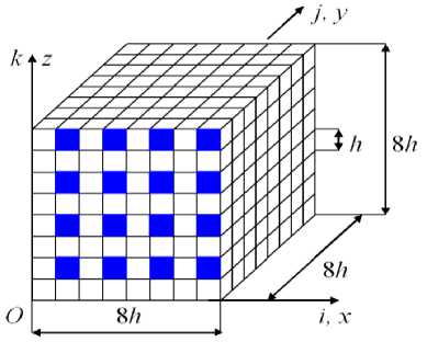
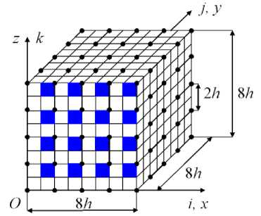
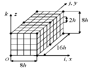
|δ| ≤δ p p n1p + n2p where ∆n =| n2p - n1p |, n1p , n2p are given; δ – relative error for voltage σb , i. e. σb - σb δ= 0 , σb where σ0 is the maximum equivalent stress of the structure Vb corresponding to the exact solution to the problem of elasticity, stresses σ0 , σb are determined by the 4th theory of strength, δp is the estimate for the error δ . Let the structure safety factor nb corresponding to the approximate solution satisfy the adjusted strength conditions of the form n1p 1 - δp np ≤n ≤ 2 b 1 + δp . where nb = σT / σb , σ – yield stress. Then the structure safety factor n0 corresponding to the approximate solution satisfies the adjusted strength conditions (14), where n0= σ / σ0 . Proof. From (16) it follows a = (1 + S) a0. From here we have nb = (1+ S)nb. Note that in (15) Cp < 1. Let So have the value that So = | S |. Then by reason of (15) we have the following formula 0 Taking into account (18) in sequence S = -So , S = So , we introduce the factors nd = (1 - So)пь, n2 = (1 + So)nb,(20) Then by the reason of (18), (20) we get nb = n^ or nb = n2.(21) Let us introduce the factors n1d , n2d according to the formulae nd = (1 - Sp) nb, nd = (1 + Sp) nb.(22) Since 0 < Sp < 1, nb > 0, from (22) it follows nd > nd .(23) Let the strength conditions (17) be satisfied for the factor n , i.e. let np < (1 - Sp)nb, (1 + Sp)nb < np. Then for the factors n1d , n2d taking into account (23) there are the following inequalities np < nd < nd < n2 . Comparing (20), (22) taking into account (19), there are the following inequalities n1d < nr , nr< nd . It follows from here that taking into account that according to (19) n^ < n2, we get nd < nr < n2 < nd .(25) Then by reason of (24), (25) there are the following inequalities np < nr < n2 < n2P .(26) From (26) taking into account (21) the fulfillment of the specified strength conditions (14) for the safety factor n0 follows. The constraints on the parameter Sp are found from the assumption of the existence of strength conditions (17), i. e. let whence it follows n1p n2p 1 - Sp 1 + Sp . Sp< Cp An . np + n2p Note that as n2p > nf > 1, then from (28) it follows 0 < Cp< 1. If Sp = Cp , then the range for varying the values of the factor nb equals to zero, i.e., in this case nb= (np + np)/2 what is difficult to perform in practice at the given n1p, n2p . Thus, at Sp< Cp it is possible to perform the given strength conditions (14) for the factor n0 with the application of the adjusted strength conditions (17) and the approximate solution that generates for the stress ab such an error S that| S| < Sp . The theorem 2 is proved. Corrected equivalent strength conditions taking into account the error of stresses. In practice, to solve the problems of the theory of elasticity formulated for three-dimensional composite structures, numerical methods are used, for example, FEM [10–12], which generate solutions with a small error. In this regard, it becomes necessary to take into account the error of solutions in equivalent strength conditions. In [16], equivalent strength conditions are considered without taking into account the error of approximate solutions. Using the results of [4], and based on Theorems 1 and 2, we formulate the adjusted equivalent strength conditions that take into account the error of the solutions. The adjusted equivalent strength conditions are reflected in the following theorem, which uses the notation introduced in Theorems 1, 2. Theorem 3. Let the equivalent strength conditions of the form be determined for the safety factor of an elastic isotropic homogeneous structure V b n1p ≤ nb0 ≤ n2p , (29) where n1p , n2p are given (i. e. the parameter p is defined, see the theorem 1); n0 – the safety factor of the structure V b corresponding to the exact solution to three-dimensional elasticity problem (formulated for the structure V b ). Let for the structure V b the maximum equivalent stress σ (corresponding to the approximate solution to the elasticity problem) be defined. Let |δ| ≤δ<C = ∆n , (30) p p n1p + n2p where ∆n =| n2p - n1p |, δ – relative error for the stress σ , i. e. δ= (σ -σ0) /σ0 , where σ0 – maximum equivalent stress of the structure Vb corresponding to the exact solution to the elasticity problem, δp – the estimate for the error δ . Let the safety factor n of the structure corresponding to the approximate solution satisfy the adjusted equivalent strength conditions of the form n1p 1 - δp np ≤n ≤ 2 b 1 + δp where n = σ / σ , σ – yield stress. Then, the safety factor n0 of the structure corresponding to the exact solution satisfies the equivalent strength conditions (29), where n0=σ /σ0 . The proof of the Theorem 3 is similar to the proof of the Theorem 2. Note that δp can be considered as the maximum error for the maximum equivalent structural stress. The relations (31) can be represented as n1p(1+ε1)≤nb ≤n2p(1-ε2), or taking into account (13) we have pn1(1+ε1)≤nb ≤ pn2(1-ε2), (32) where the values ε , ε are defined with the help of the error δp of the stress σb according to the formulae ε1 = 1 -1, ε2 =1- 1 , 0≤δp<1, (33) 1 1 - δp 2 1 + δp p – equivalence coefficient. The fundamental principles of the method of equivalent strength conditions. Let us consider a cantilever composite beam V0 having a regular structure (which is located in the Cartesian coordinate system Oxyz) with the length L = 1536h = 600 , square section that has dimensions H ×H , where H = 128h = 50 , fig. 1. The beam V0 consists of plastic materials and has static load- ing qz(x,y,z). Fig. 1. The characteristic sizes of the beam V Рис. 1. Характерные размеры балки V The regular cell Go of a composite beam Vo has the dimensions 8h x8h x 8h in which longitudinal fibers with the cross section h x h are located, fig. 2, the cross sections of the fibers are shaded, 16 fibers. Thus, the beam is reinforced with longitudinal fibers - the section h x h, the distance between the fibers is h . The fibers are isotropic homogeneous bodies and have the same elastic moduli. Fig. 2. Regular cell G0 Рис. 2. Регулярная ячейка G0 It is believed [17], if the fiber thickness is less than 0.5 mm, then such fibers form a micro-inhomogeneous structure. Let L = 600 мм, H = 50 мм, then, h = 0,3906 mm, i. e., the beam Vo with the dimensions 5 см x 60 см x 5 см has a microinhomogeneous regular fibrous structure. For the safety factor n0 of the composite beam V0 , the conditions of strength of the form (5) are specified. It is required to determine the safety factor n0 of the given beam, i.e., check whether the beam satisfies the specified strength conditions. To solve this problem, we use the method of equivalent strength conditions, the fundamental principles of which will be considered (for simplicity, without losing the commonality of views) using an example of the beam V0 with a microinhomo-geneous regular structure. The basic regular partition R0 of the beam V0 consists of (basic) singlegrid FE (1gFE) Vjh of the 1st order cube shapes with the side h [8] in which three-dimensional strain-stress state is realized. The partition R0 takes into account the microinhomogeneous structure of the beam, generates a uniform fine (base) grid with the step h of the dimension 129 x1537 x129 and a discrete model with a total number of unknown nodal FEMs Nо = 76681728, the width of the ribbon of FEM system of equations (CS) equals b0 = 50316 . The implementation of FEM for the base model R0 (more than 76 million nodal variables) requires large computer resources. The construction of a sequence of solutions is associated with the appli- cation of the grinding procedure for the basic partition, which is complex and difficult to implement for the composite structure of the beam V , since each grinding step leads to a sharp increase in the dimension of the discrete problem. Note that the step of the basic regular splitting R of the composite beam V cannot be larger than h , since the fiber cross section has the dimensions h x h. According to MESC, we introduce an isotropic homogeneous beam Vb such that the beams Vb , V have the same shape, dimensions, specified fastening and loading, but differ in elastic moduli. The elastic moduli of the beam Vb are equal to the elastic moduli of the fiber of the beam V . The implementation of MESC reduces to constructing the adjusted equivalent strength conditions (32) and to determining safety factor n of the body Vb , i. e., to determining the equivalence coefficient p for the beam V and to determining the maximum equivalent stress <r6 for the body Vb using FEM with the error 5p. The coefficient p is determined by the formula p = (r0 / сть, where <70 , ^ are the maximum equivalent stresses of the bodies Vo , Vb , respectively. Note that finding the stress <r0 by FEM (using single-grid FE cube shapes with side h [8]) for the beam Vo , taking into account its microinhomogeneous structure, requires large computer resources. The following procedure is proposed to find the equivalence coefficient p and stress сть . For the isotropic homogeneous body Vb , we construct a sequence of basic regular partitions (discrete models) {V0}N consisting of basic 1gFE V(n) of the first order of the shape of a cube with the side hn. The discrete model V0 has a dimension nx(n) x n(n) x n(n), where n(n) = 8n +1, n2n) = 96n +1, n(n) = 8n +1, n = 1,..., N. (34) The base grid steps on the axis Ox , Oy , Oz are h(n) = H/(8n), h^) = L/(96n), hzn) = H /(8n), as L = 12H, то hn= hxn) = h(yn) = hzn) and hn > h , n = 1,...,N -1. It should be noted that at n = N we get hN = h (for the law of splitting (34) at N = 16 we have h6 = h ), i. e. at n = 16 of the dimensions of an isotropic homogeneous discrete model Vx0 and basic partition R0 of the composite beam V0 are equal. It is important to note the following. The grinding law for partitions is specified so that each partition V0 consists of a finite number of areas Gb of the same shape and size that the area Gb and the area of the regular cell (Fig. 2) have the same shape, but differ in characteristic sizes. For a given grinding law (34), the area Gb has dimensions 8hn x 8hnx 8hn. The area Gb differs from the area of the regular cell G0 (in dimensions 8h x8h x8h, Fig. 2) by the characteristic dimensions of the form hn = Pnh , where Pn > 1. At n ^ 16 we have Pn ^ 1, at n = 16 we get P16 = 1 We introduce the area G0 whose shape and characteristic dimensions coincide with the area Gb, n = 1,..., N. In this case, the area G0 has a composite structure, which apparently coincides with the structure of a regular cell G0 , i.e., the area G0 has the same number of fibers (with a square section in size hn x hn ) and the same mutual arrangement as in the cell G0 (16 longitudinal fibers, fig. . 2). The fibers in the areas G0 , G0 have the same moduli of elasticity. The areas G0 , Gо , in fact, differ only in scale, that is, it can be formally written G0 = в Go, where Pn is the scale factor, Pn > 1, n = 1,...,N -1. At n = N we get PN = 1, i. e. G0 = Go. For the grinding law (34), at n = 16 we have β = 1, i.e. G0 = G . Note that the inhomogeneous (fibrous) structure is taken into account in the area G0 . In the discrete model V0 , we replace all homogeneous isotropic areas Gb with the composite areas G0 . As a result, on the basis of an isotropic homogeneous model V0 , we get a composite (base) discrete model, which we denote by R0 (in which the inhomogeneous structure is taken into account). Thus, at n = 16 the composite discrete model R0 coincides with the basic model R of a composite beam V , i.e., we have R0= R . The discrete models V0 , R0 have the same shape, characteristic dimensions, the same fastening and loading, but differ in elasticity moduli. According to (34), the dimensions of the models V0 , R0 increase sharply with increasing n . To lower the dimension of discrete models, multigrid finite elements are effectively applied [10, 11, 13, 14]. Using m - grid FEs in discrete basic models V0 , R0 we get m– grid discrete models Vb , R respectively, which have the same shape, characteristic dimensions, the same fastening and loading like the beam V , but they differ in elasticity moduli of the basic models V0 , R0 . The procedure for determining the equivalence coefficient is as follows. For the discrete models V b , R , we determine respectively the maximum equivalent stresses σb , σ , with the help of which we find the coefficient pn =σn /σnb, n = 1,..., N . We have pn → p at n →N . Let δn =| pn - pn-1 | /pn be a small value, then we have p = p . Let the sequence of solutions {σb }12 be constructed that quickly converges to an exact solution and let δσ =| σb - σb | /σb be a small value. Then we consider that σb is a maximum equivalent stress of an isotropic homogeneous body Vb (found with the error δp ). Plugging the obtained p , δp and the given factors n , n in (32), we determine the adjusted equivalent strength conditions for the composite beam V0 . The safety factor nb for the body V b is determined by the formula n = σ /σb, where σ is the yield strength of the fiber. If the found factor nb satisfies the obtained adjusted equivalent strength conditions of the form (32), then the safety factor n0 of the composite beam V0 (fig. 1) satisfies the specified strength conditions of the form (5). The results of numerical experiments. Let us consider the model problem of calculating the strength of a cantilever beam V0 with a microinhomogeneous fibrous regular structure with the dimensions 128h ×1536h ×128h, h - little, given, Fig. 1. The beam V0 consists of plastic materials, has a square section with the dimensions H ×H , where H = 128h . The regular cell of the mi-croinhomogeneous beam structure V0 with the 8h ×8h ×8h has 16 identical longitudinal fibers with a cross section h × h , Fig. 2, i. e. the beam is reinforced with isotropic homogeneous longitudinal fibers - section h × h, the distance between the fibers is h . At y = 0 : u = v = w= 0, i.e. in the plane xOz , the beam V0 is fastened. For the safety factor n0 of the beam V0 the strength conditions of the form are given 1,3≤n0≤3,2. (35) For the beam V we use the following basic data: h =0,3906; σT =5; Ev =10, Ec =1, νc =νv =0,3, qz =0,0018, (36) where Ec , Ev (νc , νv ) - Young's modulus (Poisson's ratio) of a binding material and fibers, respectively, σ - fiber yield strength, loading q acts on the surface z = H , 0,5L ≤ y ≤ L , fig. 1. To calculate the beam V we use the equivalent strength method using multigrid finite elements. In the calculations, we use homogeneous and composite Lagrangian three-grid FEs (3gFE) having the shape of a rectangular parallelepiped. We will consider the fundamental principles for constructing 3gFE using the example of a composite 3sFE V(3) having the shape of a rectangular parallelepiped with the dimensions 8h x16h x8h [10, 15]. 3gFE V(3)is located in the local Cartesian coordinate system Oxyz, which contains two regular cells Go with the dimensions 8h x8h x8h of the composite beam V . First, we consider the procedure for constructing a composite Lagrangian two-grid FE (2sFE) Vp) with the dimensions 8h x8h x 8h that contains one regular cell Go . In the procedure we use a uniform fine mesh hd with the step h and the dimensions 9 x 9 x 9 the course mesh Hd nested in the fine mesh, Hd c hd. Fig. 3 shows a fine mesh hd and a course mesh Hd having 125 nodes, which are marked with dots. The fine mesh h is generated by the basic R 2gFE V(2) , which consists of 1gFE Vh of the 1st order cube shape with the side h (in which threedimensional strain-stress state is realized, j = 1,...,M , M is the total number of 1gFE, M = 512) and which takes into account the microinhomogeneous structure of 2 gFE V(2) . The fibers are parallel to the axis Oy , the cross sections of the fibers in the plane are shaded, 16 fibers, Fig. 3. Fig. 3. Small and large mesh 2gFE V(2) Рис. 3. Мелкая и крупная сетки 2сКЭ V(2) The full potential energy P of the base partition Rd 2gFE V(2) is presented [5; 8] 512 П=E (7 qT [ Kh hj- qTP). (37) .I=12 where [Khj ] – stiffness matrix, Pj , q j– the vectors of nodal forces and displacements of 1gFE Vjh of the base partition 2gFE, T – transposition. Using Lagrange polynomials [5] on the large mesh Hd we define approximating displacement functions u ,v ,w for 2gFE V(2) , which are written in the form 555 555 555 u2 =ZZZNjkUjk , V2 =ZZZNukvyk , w2 =ZZ2N , (38) i=1 j"=1 k=1 i=1 j"=1 k=1 i=1 j=1 k=1 where uijk, vijk , wijk – displacement values u, v, w in the node i, j,k of the mesh Hd ; i, j,k – coordinates of an integer coordinate system ijk , introduced for the mesh nodes Hd (fig. 3); Nik = Nijk(x, y,z) - base function of the node i, j, k of the mesh Hd , i, j,k = 1,...,5 , Nijk = Li(x)Lj(У)Lk(z), where Li(x)= ∏5 x-xα , Lj(y)= ∏5 y-yα , Lk(z)= ∏5 z-zα , (39) α=1,α≠i xi - xα α=1,α≠ j yj - yα α=1,α≠k zk - zα xi,yj,zk – coordinates of the node i, j,k of the mesh H in the coordination systemт Oxyz , fig. 3. Let us denote: Nβ = Nijk, uβ = uijk , vβ = vijk , wβ = wijk, where i, j,k =1,...,5 , β =1,...,125. Then the equations (38) take the form 125 125125 u2=∑Nβuβ, v2=∑Nβvβ, w2=∑Nβwβ.(40) β=1 β=1 We denote by qd = {u1,...,u125, v1,..., v125, w1,..., w125}T nodal displacement vector of the mesh H , i. e. nodal unknown vector 2gFE V(2) . Using (40), the components of the vector qj of the nodal variables 1gFE Vh are expressed in terms of the components of the vector q , as a result we get the equation qj =[A2j] qd,(41) where [A2] – rectangular matrix, j = 1,...,512 . Substituting (41) into equation (37), from the condition ∂П /∂q = 0 we get [K ] q = F , where 512512 [Kd]=∑[A2j]T[Khj][A2j], Fd=∑[A2j]TPj,(42) j=1 where [Kd ] – stiffness matrix (the dimension – 375×375), Fd – nodal force vector (the dimension – 375) 2gFE V(2). Let us consider the construction of the Lagrangian three-grid FE (3gFE) Vα(3) , using two 2gFE V (2) . The small mesh hα and the large one Hα of 3gFE V(3) are shown in fig. 4, the nodes of the mesh Hα are marked with dots, 12 nodes. The nodes of the small mesh hα are the nodes of the large meshes Hd of two 2gFE V(2) , d = 1, 2 . Fig. 4. Small hα and large Hαmesh 3gFE Vα(3) Рис. 4. Мелкая hα и крупная Hα сетки 3сКЭ Vα(3) The full potential energy P 3gFE Vα(3) can be presented in the form Pα=∑(1qTd[Kd]qd-qTdFd), (43) d =1 2 where [Kd ], Fd, qd – stiffness matrix, vectors of nodal forces and displacements 2gFE Vd(2),d=1, 2. Using Lagrange polynomials on the large mesh Hα we determine the approximating functions of displacements u ,v ,w for 3gFE V(3) , that are written in the form 232 232 232 u3=∑∑∑Nijkuijk, v3=∑∑∑Nijkvijk , w3=∑∑∑Nijkwijk, (44) i=1 j=1 k=1 i=1 j=1 k=1 i=1 j=1 k=1 where uijk, vijk, wijk – displacement values of u, v, w in the node i, j,k of the mesh Hα; i, j,k – coordinates of an integer coordinate system ijk , introduced for the mesh Hα (fig. 4); Nijk = Nijk(x, y, z) – base function of the node i, j,k of the mesh Hα, i,k = 1,2, j = 1,2,3 , Nijk = Li(x)Lj(y)Lk(z), where 23 2 Li(x)= ∏ x-xα , Lj(y)= ∏ y-yα , Lk(z)= ∏ z-zα , (45) α=1,α≠i xi - xα α=1,α≠ j yj - yα α=1,α≠k zk - zα xi,yj,zk – node coordinates i, j,k of the mesh Hα in the coordinate system Oxyz , fig. 4. let us denoteNβ =Nijk, uβ =uijk, vβ =vijk, wβ =wijk, where i,k=1, 2, j=1, 2, 3, β = 1,...,12 . Then the equations (44) take the form 12 1212 u3=∑Nβuβ, v3=∑Nβvβ, w3=∑Nβwβ.(46) β=1 β=1 We denote by q = {u ,...,u , v ,..., v , w ,...,w }T the vector of nodal displacements of the large mesh Hα, i.e., the vector of nodal variables 3gFE V(3) . Using (46), the vector components q of nodal variables 2gFE V (2) are expressed by the vector components qα , as a result we get qd =[Ad3] qα,(47) where [A3] – rectangular matrix, d = 1, 2 . Substituting (47) into the expression (43), from the condition ∂P /∂q = 0 we get [Kα] qα=Fα, where 22 [Kα]=∑[Ad3]T[Kd][Ad3], Fα=∑[Ad3]TFd ,(48) d=1 where [Kα] – stiffness matrix (the dimension-36×36), Fα - nodal force vector (the dimension – 36) 3gFE Vα(3) . Comment 2. The solution built for the large mesh Hα 3gFE Vα(3) , using the formula (47) is projected onto the small mesh hα 3gFE Vα(3) . Then, using the formula (41), we determine the nodal displacements of the basic partitions 2gFE V(2) , which makes it possible to calculate stresses in any 1gFE Vjh of base partition Rd 2gFE V(2) , d = 1, 2 . Comment 3. By virtue of (41), the dimension of the vector qd (i.e. the dimension of 2gFE V(2) ) does not depend on the total number M of 1gFE Vjh , i.e. on the dimension of the partition Rd . Therefore, to take into account the microinhomogeneous structure in 2gFE, one can use arbitrarily small basic partitions consisting of 1gFE Vjh . In this case in 2gFE V(2) (consequently, in 3gFE Vα(3) ) the three-dimensional strain-stress state is described arbitrarily accurately (without introducing additional simplifying hypotheses). Using the procedures described in [14], 2gFE are designed to calculate composite shells of revolution, rings of complex shape and shafts that have central circular holes, composite and uniform cylindrical shells, plates and beams of complex shape, which are widely used in practice. The procedure for constructing homogeneous multigrid finite elements is similar to the procedure for constructing composite multigrid finite elements. For the composite beam V we define an isotropic homogeneous body Vb (the beam Vb ). The bodies V , Vb have the same shape, size, fastening and loading, the elastic moduli of the body Vb are equal to the elastic moduli of the fiber. Using the law of splitting (34), we construct, according to the procedure described above, three-mesh discrete models Vb , R , consisting respectively of isotropic homogeneous and composite 3gFE of the type V(3) with the dimensions 8hn x 16hn x 8hn , n = 1,12. For the discrete isotropic homogeneous model Vb we find the solutions wb , cb , where wb, ob - maximum displacement and equivalent voltage of the discrete model Vb, n = 1,...,12. Equivalent stresses are determined by the 4th theory of strength. The calculation results are presented in Table 1. The analysis of the calculation results shows a fast uniformly monotonic convergence of approximate solutions ( wb, Ob ) to the exact solution. The stresses ob = 0,665, ob = 0,686, differ by 5 = 3,061%. The test calculations show that in this case the stress ob is found with the error 10% ^15%. Let 5p = 0,15 . The condition (30) for 5p is satisfied. Taking into account relations (13) and (35) in (30), we have 5p = 0,15 < Cp = 0,42. According to (33) at 5p = 0,15 we get ^ = 0,176, ^2 = 0,131. The adjusted equivalent strength conditions (32) for ^ = 0,176, ^2 = 0,131 have the form 1,176pn1< nb< 0,869pn2, (49) where n - safety factor of the body Vb , determined by FEM. Таблица 1 The results of calculations of the beam Vb Результаты расчетов балки Vb Vnb b n °bn Vnb b n °bn V1b 204,851 0,377 V7b 238,033 0,569 V2b 228,503 0,489 V8b 238,263 0,595 V3b 234,023 0,524 V9b 238,422 0,620 V4b 236,109 0,537 b V10 238,545 0,643 V5b 237,119 0,543 b V11 238,630 0,665 V6b 237,683 0,547 b V12 238,697 0,686 Note that the three-grid discrete model V1 2, consisting of Lagrangian 3gFE of the type V^3^ (a = 1,...,32768) with the dimension 8h2x16hx2x8hx2, has Nb2= 73008 of nodal variables of FEM, the width of the tape the control system of FEM is b2 = 1059 . The implementation of FEM b - , N xb 76681728x50316 for the discrete model V2 requires k = —0---— =----------------= 49903,566 times less com- 12 Nb x b2 73008 x1059 puter memory than for the base model R0 of the beam V0 , which shows the high efficiency of the application of Lagrangian 3gFE of the type V^in the calculations. The equivalence coefficient p for the composite beam V0 is determined using the procedure described above. The discrete models Vb, Rn, n = 9,11,12 are constructed using 3gFE of the type V(3) based on basic regular partitions, respectively, with the dimensions: 73 x 865 x 73, 89 x1057 x 89 и 97 x1153 x 97. The equivalence coefficients pn are found by the formula pn = ^ / ^b, where <r„ , ab - maximum equivalent stresses of the models Rn, Vb, n = 9,11,12 respectively. As a result of the calculations, we get: p9 = 3,002, p- j = 3,000, px2 = 2,999 . The relative errors for the found coefficients p9 , px p p12 are §1 (%) = 100%x | p11 - p9 |/ p11 = 100%x |3,002 - 3,000| / 3,000 = 0,066% , 52 (%) = 100%x | p22 - p11|/ p12 = 100%x 13,000 - 2,9991 / 2,999 = 0,033%. As p9 > px j > p12 and § is the smallest value, then we assume that the equivalence coefficient is p = p12= 2,999. Plugging into (49) p = 2,999, n1 = 1,3, n2= 3,2, we get 4,584 < nb< 8,339. (50) The safety factor of the homogeneous body Vb is nb = ^ / ab = 5/ 0,686 = 7,288, which satisfies the adjusted equivalent strength conditions (50). This means that the safety factor n of the composite beam V satisfies the specified strength conditions (35). Let us perform verification calculations. Based on the underlying partition R of the beam V using 3gFE V(3) we build three-grid discrete models: composite R and isotropic homogeneous Rb corresponding to the law of splitting (34) at n = 16. We consider that the stresses <r16 = 2,279, ob = 0,762 correspond to exact solutions, i.e. cr0= ^6, ab = ab. Then the safety factor for the composite body Vo is n0 = <тг / cr0= 5/2,279 = 2,194, i.e. n0 = 2,194 satisfies given strength conditions (35), which confirms a similar conclusion obtained using MESC. The equivalence coefficient p (corresponding to the exact solutions) for the beam V is p0 = (70 / The dimension of the base discrete model V10 (whose mesh at n = 12 has the dimension 97 x1153 x 97, see formulae (34)) equals 32517504, the width of the tape of the control system of FEM is 28524. The number of nodal variables of FEM of the three-grid discrete model V1b2 equals 73008, the width of the tape of the control system of FEM is 1059. The implementation of FEM for a homogeneous isotropic three-grid discrete model V1b2 requires k 2 = 32517504 x 28524 73008x1059 = 11996,685 times less computer memory than for the base model V12 , consisting of the known 1gFE of the cube shape with the side h . Conclusion. The method of equivalent strength conditions is proposed for calculating the static strength of structures (plates, beams, shells) with an inhomogeneous, microinhomogeneous regular structure under specified strength conditions. The implementation of the method is reduced to calculating the strength of isotropic homogeneous bodies with the use of equivalent strength conditions built on the basis of given ones. When calculating homogeneous bodies according to FEM, multigrid finite elements are used, which generate discrete models of small dimension and solutions with a small error. The implementation of the proposed method requires small computer resources.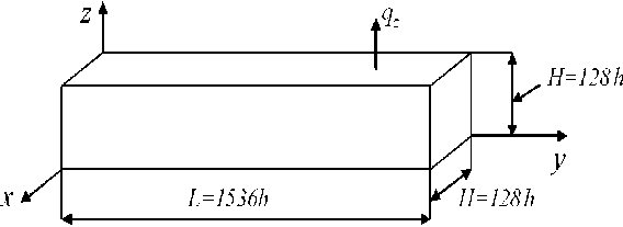
References The method of equivalent strength conditions in calculating composite structures with a regular structure using multigrid finite elements
- Pisarenko G. S., YAkovlev A. P., Matveev V. V. Spravochnik po soprotivleniyu materialov [Handbook of resistance materials']. Kiev, Nauk. Dumka Publ., 1975, 704 p.
- Birger I. A., SHorr B. F., Iosilevich G. B. Raschet na prochnost' detaley mashin [Calculation of the strength of machine parts]. Moscow, Mashinostroenie Publ., 1993. 640 p.
- Moskvichev V. V. Osnovy konstrukcionnoy prochnosti tekhnicheskih sistem i inzhenernyh sooruzheniy [Fundamentals of structural strength of technical systems and engineering structures]. Novosibirsk, Nauka Publ., 2002, 106 p.
- Matveev A. D. [Calculation of elastic structures using the adjusted terms of strength]. Izvestiya AltGU. Matematika i mekhanika. 2017, No. 4, P. 116–119 (In Russ.). Doi: 10.14258/izvasu(2017)4-21.
- Norri D., de Friz Zh. Vvedenie v metod konechnykh elementov [Introduction to the finite element method]. Moscow, Mir Publ., 1981, 304 p.
- Golovanov A. I., Tiuleneva O. I., Shigabutdinov A. F. Metod konechnykh elementov v statike i dinamike tonkostennykh konstruktsii [Finite element method in statics and dynamics of thin-walled constructions]. Moscow, Fizmatlit Publ., 2006, 392 p.
- Obraztsov I. F., Savel'ev L. M., Khazanov H. S. Metod konechnykh elementov v zadachakh stroitel'noi mekhaniki letatel'nykh apparatov [Finite element method in problems of aircraft structural mechanics]. Moscow, Vysshaia shkola Publ., 1985, 392 p.
- Zenkevich O. Metod konechnykh elementov v tekhnike [Finite element method in engineering]. Moscow, Mir Publ., 1975, 544 p.
- Fudzii T., Dzako M. Mekhanika razrusheniya kompozicionnyh materialov [Fracture mechanics of composite materials]. Moscow, Mir Publ., 1982.
- Matveev A. D. [The method of multigrid finite elements in the calculations of three-dimensional homogeneous and composite bodies]. Uchen. zap. Kazan. unta. Seriia: Fiz.-matem. Nauki. 2016, Vol. 158, Iss. 4, P. 530–543 (In Russ.).
- Matveev A. D. [Multigrid method for finite elements in the analysis of composite plates and beams]. Vestnik KrasGAU. 2016, No. 12, P. 93–100 (In Russ.).
- Matveev A. D. Multigrid finite element method in stress of three-dimensional elastic bodies of heterogeneous structure. IOP Conf, Ser.: Mater. Sci. Eng. 2016, Vol. 158, No. 1, Art. 012067, P. 1–9.
- Matveev A. D. [The construction of complex multigrid finite element heterogeneous and microinhomogeneities in structure]. Izvestiya AltGU. Matematika i mekhanika. 2014, No. 1/1, P. 80–83. Doi: 10.14258/izvasu(2014)1.1-18.
- Matveev A. D. [Construction of multigrid finite elements to calculate shells, plates and beams based on generating finite elements]. PNRPU Mechanics Bulletin. 2019, No. 3, P. 48–57 (In Russ.). Doi: 10/15593/perm.mech/2019.3.05.
- Samul' V. I. Osnovy teorii uprugosti i plastichnosti [Fundamentals of the theory of elasticity and plasticity]. Moscow, Vysshaia shkola Publ., 1982, 264 p.
- Matveev A. D. [Strength calculation of composite structures using equivalent strength conditions]. Vestnik KrasGAU. 2014, No. 11, P. 68–79 (In Russ.).
- Golushko S. K., Nemirovskii I. V. Priamye i obratnye zadachi mekhaniki uprugikh kompozitnykh plastin i obolochek vrashcheniia [Direct and inverse problems of mechanics of elastic composite plates and shells of rotation]. Moscow, Fizmatlit Publ., 2008, 432 p.
