The money market model simulation on the example of the Russian Federation

After a decade since creation the new economic system, Russian economy has experienced rapid growth. The beginning of it was initiated by the process of import substitution in the domestic market after the crisis of 1998 and ruble devaluation. Now we can use collected data for analytical goals. The purpose of this study is to analyze the factors that determine changes in the degree of economic growth in Russia. For those purposes we chose Money market model that represents econometric expression of dependence of GDP, domestic investments, interest rates and money supply.

Determination of variables

Determination of variables is the first step of econometric modeling. There are two possible kinds of econometric variables: endogenous (internal and dependent) and exogeneous (external and independent). Initially in the money market model two endogenous variables are considered – interest rate and GDP. After specification process, we expressed one endogenous variable that we are interested in: GDP and two exogenous variables: money supply and domestic investments. Thus, GDP values are internal and are explained by our econometrics model [1].

Statistical data description volume of domestic investment, ordinary least

In order to analyze and test GDP development, we need to collect time series data from reliable statistic resources: the volume of GDP in billions of USD, which denoted as Yt; the volume of money supply in billions of USD, which denoted as Mt; and the volume of domestic investment in billions of US dollars, which denoted as It. Data was taken annually because of the specificity of the country's macroeconomic reporting. As source for GDP and Domestic investment numbers we used World Bank national accounts data [2]. According to World Bank, Gross domestic fixed investment now explained as Gross fixed capital formation in data bank [3]. Money supply was taken from the Central Bank of the Russian Federation [4]. Initial table with data is represented in the Application 1. The indicators are taken for the period from 2000 to 2017 as the biggest possible period without heteroscedasticity.

Analysis of the scatter diagram

In order to analyse dependence between variables we need to build the scatter plot. It displays the actual values along the X-axis, and predicted values along the Y-axis. Also, it displays a line that illustrates the perfect prediction, where the predicted value exactly matches the actual value. The distance of a point from this ideal 45-degree angle line in- performed [5]. dicates how well or how poorly the prediction

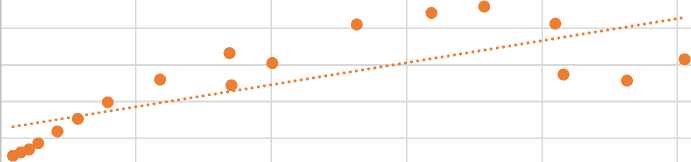
Y=f(M)

y = 0,0006x + 627,82

R2 = 0,5748

0,00       500000,00    1000000,00    1500000,00   2000000,00   2500000,00   3000000,00

M, bln USD

Pic. 1. Scatter diagram. The dependence of GDP from Money supply

On the first diagram R2 is close to 0,575, it means that 57,5% of total deviation of Y is explained by the M variation by linear regression model. But we can see large spread of predicted values far from actual value line. Picture 1 illustrates a scatter diagram where M is an increasing function of Y and the heteroscedasticity is presented.

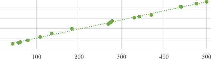
Y=f(I)

y = 4,4188x + 91,421

R2 = 0,9962

I, bln USD

Pic 2. Scatter diagram. The dependence of GDP from Domestic investment

On the second diagram R2 is close to 0,996, it means that 99,6% of total deviation of Y is explained by the I variation by linear regression model. As R2 is close to 1, hence variable I does describe Y by linear regression model with very high accuracy. Picture 2 il- lustrates that variables have the same finite variance and the homoscedasticity is presented [6].

Correlation analysis

To make a full correlation analysis we need to construct correlation matrix.

Table 1. Correlation matrix

	I, bln USD	M, bln USD	Y, bln USD
I, bln USD	1
M, bln USD	0,758	1
Y, bln USD	0,998	0,758	1

From the table we can see that corr(Y, I) between GDP and domestic investment is 0,99 and corr(Y, M) between GDP and mon- ey supply is 0,76. Both indicators have a strong positive linear relationship via a firm linear rule. When money supply or domestic investment increases, the GDP increases too and vice versa.

Correlation analysis shows that GDP of Russia positively but with heteroscedastic results depends on Money supply and strongly and clearly depends on Domestic investment.

Econometric model specification.

Development of the model begins with the specification of the model, which is a detailed description of the object of research followed by the representation of the process of its functioning in the form of mathematical formulas. Initial form for capital market model was made with needs of the principles of specification.

First, the Money market model emerged from the translation of economic statements into mathematical language. It was taken as part of IS–LM macroeconomic model, or Hicks–Hansen model. It describes interaction between interest rates and GDP in dependence with investments, savings, money demand and money supply on the market. Second, model has two equations as it has two endogenous variables. Third, the model is dynamic and consider time influence. Forth, the model takes into account random variables [7].

Money market model initial form:

R _t = a₀ + d i M_t + a.₂Y_t + £_t Y_t = bo + b^R _t + b₂I_t + v_t

E(8t) = 0; E(v_t) = 0 a (ft) = const; o"(v_t) = const

After some calculations we reached an equation of the reduced form of the model:

Y_t = (b o + b i • « o + b«a₀ •Mt + b i • c_t + b₂ • I_t + v) • —i— (2)

Г       ^z Г       ^ty i - b i• a2 ^{v 7}

For purposes of estimation we have prepared a new reduced form equation with replaced coefficients:

Y_t = A o + A i • M t + A 2 • I_t + c_t (3)

Estimating the coefficients of the model in Excel

After data preparation we can make the regression analysis. The correlation analysis may show dependencies but not showing us if model is correct. To estimate it, we will take data from 2000 to 2017 and make Regression in Excel with 95% level of significance.

Here we will represent regression analysis in the finished form of Money market model, but we need to notice that we discovered that coefficient and standard error before Money supply approaches zero. Further, after multiple normalization attempts and estimating we discovered that t crit always higher than t stat . From this analysis we decided to exclude Money supply from the model as insignificant.

The results of regression statistics with two remaining variables are following:

Table 2. Summary output
Regression Statistics
Multiple R	0,998
R-square	0,996
Adjusted R-square	0,996
Standard Error	43,08
Observations	18

Table 3. Analysis of variance

	df	SS	MS	F	Significance of F
Regression	1	7758912,32	7758912	4180,4	8,79E-21
Residual	16	29696,32	1856,02
Total	17	7788608,64

Table 4. Regression coefficients

	Coefficients	Standard error	t-stat	P-value	Lower 95%	Upper 95%
Y-intersection	91,42	20,41	4,48	0,00	48,16	134,68
It	4,42	0,07	64,66	0,00	4,27	4,56

Specification of the estimated model

After first step of regression analysis we can make an estimated model:

Y_t = 91, 42 + 4,42∙ I_t + s_t

(20,41)

[4,48]

R² = 0,996

(0,07)  (43,08)

[64,66]

Peril = 4180,4

All numbers from first equation demonstrates λ-coefficients. Numbers in the round brackets shows standard error for every coefficient and random variable. Numbers in square brackets represents t-statistic [8].

Received coefficients shows how dependent variable would react if independent variable changes. λ 0 = 91,42 shows that GDP will be equal 91,42 bln of USD if domestic investment is equal to zero. λ 1 = 4,42 implies that if domestic investment is growing by 1%, GDP would increase by 4,42 bln of USD or if domestic investment is decreasing by 1%, GDP would decline 4,42 bln of USD.

Model testing

After making the regression analysis we need to test our model with R2-test, F-test, t-test, Goldfeld-Quant test and Durbin-Watson test [9].

R2-test

R2 helps us to understand relevance of chosen endogenous factors in per sent. To infer about this test, we need to look at the regression analysis table and find R-square. The closer the number to one, the more accurate our model is in explaining Yt by It.

In this research, value of R-square is 99,6% which shows that GDP deviation is explained by the variation of domestic investment and significantly affected by it. This means correctness of the estimated model.

F-test

In our work F crit =4,49 < F=4180,4 so we can confirm that R-square is non-random, economic model has high quality.

t-test

T-test checks the significance of coefficient. If |t| is bigger than t crit we can say that coefficients are important. To find t crit we can use the formula T.INV.2T (0,05; residual).

We received t crit = 2,12 that is lower than t stat = 4, 48, which means that coefficient Y-intercept is significant under the probability of 5%, and t crit = 2,12 is lower than t stat = 64,66 which also means that that coefficient λ 1 is significant.

Goldfeld-Quandt test

To verify the possibility of using the ordinary least square method, it is necessary to check three conditions of the Gauss-Markov theory. GQ-test helps to detect homoscedas-ticity in regression analysis. For these purposes we should divide our data into three groups and make new regression analysis for first six and last six numbers. Ratio of the two sums of squares is our GQ, data for estimation can be found in SS column crossed with residual raw. Our newly calculated F crit = 6 > GQ = 0,19 and F crit = 6 > 1/GQ=5,29. That means our coefficients are homoscedastic unbiased, consistent, accurate.

Durbin-Watson test

This test is used to determine whether there is autocorrelation in the residuals from a regression analysis. First of all, we should check if expectation of residuals is equal to 0. For these purposes we use function AVERAGE. In this model E( 8^ )=0. After we should estimate DW statistics:

DW = ^∑ ^ ∑ ⁽ Et^{2 )} "  (5) ^∑

After calculations we received DW=0,906 and now we can find critical values d L and d U in Durbin-Watson statistic table with 1% significance, where t=18 - number of observations, k=1 – number of factors.

Table 5. DW statistics interval

0	dl (lower)	du (upper)	2	4-du	4-dl
0	0,902	1,118	2	2,882	3,098

Value of DW is in the interval between d L and d U with probability 1%. It means we don’t have information about autocorrelation in this model.

Confidence interval and the model adequacy

In order to estimate the lower and upper boundaries we should calculate Y estimated by multiplying coefficients and variables ac- cording to our model equation. For this test we should use 2017-year data.

• 1)    Y est = Л_о + Л1 ∙ It = 91,42 + 4,42 × 342,23 = 1603,65.

• 2)    Y lower = Y est – t crit × standard error = 1603,65 - 2,12 × 43,08 = 1512,325- the lower boundary;

• 3)    Y upper = Y est + t crit × standard error = 1603,65 + 2,12 × 43,08 = 1603,654 - the upper boundary.

Table 6. Y real lies in the confidence interval

Y-	Y real	Y+
1512,325	1577,52	1603,654

The real GDP value lies in the confidence interval, predicted by our model, it means that the model is adequate.

The mistake of approximation equals to 1, 63% that means that our model has high accuracy.

Mistake of approximation =

ABS ( Y real - Y estimated )

Y estimated

Economic analysis of the model results.

Model results show us that domestic investment plays significant role in sustainable development of Russia while role of money supply is minor [10]. This result is consistent with J.M. Keynes' vision and reproduce his theory. They show that even small change in investment by 1% is considered as a way to increase national income, which leads to new workers, increased employment and higher level of savings. However, the coefficient before money supply tends to zero, we should mark that according to Keynes, periodic increasing of money supply reduces interest rate which stimulates production growth [11].

Conclusions and forecast

Investigated econometric model is built according to econometric principles, is significant and did pass all tests. After analyzing it we may create several conclusions. First, correlation between domestic investment and GDP is high, as between money supply and GDP. Second, regression analysis shows that money supply is insignificant factor for current model. However, regression analysis also shows high level of significance of domestic investment, so if we took estimated model, we will see that the higher the investment into land improvements, plants, machinery, construction of roads, railways, schools and the like, the higher the Gross domestic product. Third, quality of specification is high and model is adequate.

This all shows us that Russian GDP highly linearly dependent on such factor as domestic investment and we can infer that this model is appropriate and may be applied for forecasting future GDP volumes in Russia.

Application 1

Table 1. Initial Data

	GDP, billions of US dollars	Money supply, billions of US dollars	Domestic Investment, billions of US dollars
Year	Yt	Mt	It
1993	435,08	427,49	88,71
1994	395,08	2183,48	86,17
1995	395,53	6432,05	83,37
1996	391,72	14521,44	78,35
1997	404,93	18960,74	74,07
1998	270,95	24603,58	43,76
1999	195,91	29838,67	28,18
2000	259,71	46997,38	43,8
2001	306,6	75671,97	57,91
2002	345,47	105846,05	61,86
2003	430,35	140117,45	79,25
2004	591,02	210797,67	108,66
2005	764,02	286344,68	135,65
2006	989,93	396715,53	183,17
2007	1299,71	589979,62	272,88
2008	1660,85	846360,67	370,21
2009	1222,64	853391,21	268,92
2010	1524,92	1004110,36	329,77
2011	2051,66	1316130,63	440,84
2012	2210,26	1591886,76	476,31
2013	2297,13	1786545,11	500,22
2014	2063,66	2049022,81	438,48
2015	1368,4	2079282,39	278,02
2016	1284,73	2313677,40	274,44
2017	1577,52	2526651,97	342,23