The Multifractal Analysis Approach for Photogrammetric Image Edge Detection

Data obtained from the digital images processing are very important for modern technology, science and engineering and also national economics development. Digital images processing methods are steadily being developed and upgraded in terms of image visual perception improving, its preprocessing, denoising, segmentation and classification of images in order to extract the objects of interest.

Space photogrammetric snapshots are fixed in a number of electromagnetic radiation spectral ranges, so they are multispectral images so that have their own special attributes as compared with color images in general. Such multispectral image features as different information value and different spatial resolution subject to image spectral band, time, position, optical sensor features and etc. dependencies of image forming processes affect the specialty with its processing.

The principle of image segmentation in order to analyze and classify the objects of interest in the image consists of the image separation into components or primitive objects. The detailing level of the shared areas depends on the current task. For example, when the object of interest ceases to maintain the integrity and becomes being divided into smaller parts, the segmentation process should be finished.

Image segmentation algorithms are often based on the similarities and breaks of the image intensity values. The approach of intensity breaks is based on sudden changes in image brightness values. The approach of intensity similarities is based on the image division into similar regions according to a number of pre-defined criteria. Thus, the choice of image segmentation algorithm depends on the task to be solved. The edge detection is an integral part of image segmentation techniques set as far as the effectiveness of many tasks solving of image processing and computer vision often depends on the quality of interested objects contours extracting.

The principle of multifractal based image segmentation is the following. It seems intuitively clear that points in an image can be classified according to their Hölder exponent [1]. Herewith the Hölder exponent is the regularity characteristic for intensity level distribution on the image field. The point-wise, local, Hölder exponent represents the local regularity, which is proportional to the current value of the exponent. So, let us take the example of points lying on contours. These points often correspond to discontinuities of the grey level map or of its derivative. They thus have in general "low" Hölder regularity. However, the exact value of the exponent will depend on the characteristics of the image. In addition, the property of being an edge is not purely local, and one needs a global criterion in order to decide that a given point is an edge point. Indeed, points lying in textured regions also have in general a low regularity, and one has to find a way to distinguish them from contours.

As a powerful mathematic tool, fractal theory initiated by Mandelbrot [2] has been widely applied to many areas of natural sciences. The approach of Image Multifractal Segmentation is fully nonparametric, and analyses the image through various features of its multifractal spectrum [3]. Although it is perfectly possible to use Weakly Self-Affine functions [4] to model and segment images as well as to use multifractal tools for the segmentation of 1D signals. In fact, this is really a modeling method used for segmentation purposes.

• II.    General Approaches to Image Multifractal Segmentation

Since edges are by definition sets of points of dimension one, we shall declare a point to lie on a contour if it has an exponent such that the associated value of the multifractal spectrum is one. Note that, in addition to this geometrical characterization of edge points, a statistical one is possible. Edge points may be defined by their probability of being hit when a pixel is randomly chosen in the image at a given resolution. The link between the geometrical and statistical characterizations is provided by the multifractal formalism. Starting again from the Hölder exponents, one can decide to keep those points where the spectrum has any given value. One starts by computing the Hölder exponent at each point. This yields the image of Hölder exponents. The second step is to compute the multifractal spectrum. Finally, one chooses which kind of points to extract, i.e. points on smooth edges, textures, etc..., by specifying the corresponding value of the spectrum.

The analysis is performed with respect to the Lebesgue measure; exponents are computed by comparing the content of a region with its size.

In [5] the local behavior of a continuous function is explained. A non-trivial open interval I of R is given, the local regularity at a point x ₀ E 7 of a function f E L”_oc (7) is given by the point-wise Holder exponent h^(x₀). The function f belongs to C^_o if and only if there exist a constant C and a polynomial P of degree smaller than [A] such that

Vx E 7 close enough to x₀, \f(x) - P(x - X o )| <  C\x - X o l " .

The pointwise Holder exponent of at is hf(Xo) = sup{h:f E C^}.

Multifractal analysis then focuses on the dimension of the fractal level sets of the function h , that is the sets of the form

E^ = {x E 7: hj(x) = h}, (h > 0).

The computation of the Point-wise Hölder exponent was executed by different ways of measuring the content of a given region in the image:

• -    associating to each region the sum of the grey level of the pixels in it;

• -    computing the Lp norm, i.e. the 1/p-power of the sum of the p-powers of the individual grey levels ( lpsum capacity);

• -    measuring the region content by the min imum of the grey levels of its pixels;

• -    measuring the region content by the max imum of the grey levels of its pixels;

• -    assigning to a region the cardinal of the largest subset of pixels having the same grey level ( iso capacity).

For instance, if a region is composed of N pixels all having different grey levels, its iso capacity will be one. If all pixels have the same grey level, the iso capacity is N. The adaptive iso is a refinement of this taking into account a possible noise in the image.

At the next step, the multifractal spectrum of the processed image could be computed by one of the following three algorithms, which are proposed by Fractal Theory.

The Hausdorff spectrum gives geometrical information pertaining to the dimension of sets of points in the image having a given exponent. This spectrum is a curve where the abscissa represents all the Hölder exponents that occur in your image, and the ordinate is the dimension of the sets of pixels with a given exponent.

The second spectrum is the large deviation spectrum. This spectrum yields the statistical information, related to the probability of finding a point with a given exponent in the image. The computation is based on techniques used in density estimation, and uses a kernel of optimal, signal dependent, size computed from some empirical statistical criterion.

The third spectrum is called the Legendre spectrum. It is just a concave approximation to the large deviation spectrum. Its main interest is that it usually yields much more robust estimates, though at the expense of an information loss.

According to [5] the Hausdorff dimension is the most common notion of dimension, denoted dim in the paper. The Hausdorff multifractal spectrum of is defined by df: h ^ dimE^.

During segmentation, those points the exponent of which have a corresponding value of spectrum that falls inside the definite range of dimensions are being extracted from the original image. The result is a binary image, where the extracted points are in white and everything else is black.

• III.    Hölder Exponent Based Segmentation Algorithm

The image processing feature of interest is the Hölder exponent (also known as the Lipschitz exponent). This is a scalar quantity, readily computable from the wavelet transform [6, 7], which represents the regularity or differentiability of a given signal; the higher the exponent, the higher the regularity.

The following segmentation algorithm is

• -    computing the corresponding alpha image from the normalized grayscale input image, using a specific radius and specific measure type. The radius is an integer from 1 to 5, which defines the largest measure domain. The measure methods used in the study are Maximum, Minimum, Sum, Iso, Adoptive Iso of square shaped domain.

The pixels in the alpha image are estimated values of Hölder exponent at these points and they describe the local regularity of an input image.

The Hölder exponent at the definite point is estimated from bi-logarithmic diagram ln(Mi(m, n)) vs. ln(i), where Mi(m, n) is the amount of the chosen measure within measure domain of size i at particular image pixel with spatial coordinates (m, n).

The limiting value of alpha(m, n) is estimated as a slope of the linear regression line in this log-log diagram [8, 9].

• -    carrying out the alpha image discretization thereto the alpha image is being covered by a regular grid of boxes with integer box sizes j = 1,2,4,6,8,10,12,14,16 pixels.

The size of each bin is k = (N - 1)/(max - min), where N is the number of bins, max and min are the maximum and minimum intensity levels of the alpha image.

The boxes containing at least one value of that alpha bin are counted giving the overall number of hitboxes of size j, Nj(alpha bin) for that alpha bin. Boxes of different sizes are recursively taken into account, and corresponding Hausdorff measures are calculated for each image pixel from bi-logarithmic diagram ln(Nj(alpha bin)) vs. ln(j). The limiting value of f(alpha bin) is estimated as a slope of the linear regression line in this log-log diagram.

This procedure is repeated for every of N equally sized alpha bins, obtaining the 1D f(alpha) multifractal spectrum and also the f(alpha) image filled by pixel-wise values of f(alpha).

• -    computing the multifractal Hausdorff spectrum from the alpha image using a specific number of bins, which is a positive integer. As follows the components of the

spectrum are normalized to 2 to achieve the minimum misrepresentation.

• -    computing the corresponding f(alpha) image from an input alpha image using a specific number of bins for input alpha image discretization defining.

The function f(alpha) describes the global regularity of an input image and is the result of the following segmentation process.

• IV.    Experimental Results

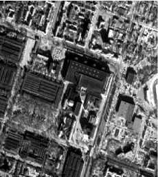
As the testing images the Ikonos panchromatic images of University campus area (fig. 1 a) and urban area (fig. 1 c), the Ikonos blue band multispectral image of University campus area (fig. 1 b) and the Ikonos NIR multispectral image of urban area (fig. 1 d) were kept. The resolution of the panchromatic images is 1 meter and the spectral range is 0.45 - 0.90 mkm. The resolution of the multispectral images is 4 meters and the spectral ranges are 0.45 - 0.53 mkm for the blue band and 0.77 -0.88 mkm for NIR band images.

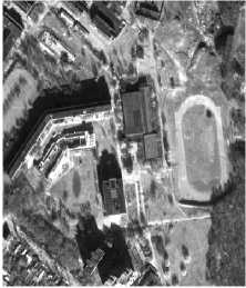
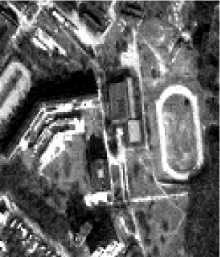
b

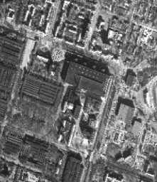
Fig.1. The initial photogrammetric images

The images obtained after segmentation process are shown below in Table I in accordance with Hölder exponent capacity provided Hausdorff Spectrum was used. Such parameters for "fat" binary image containing smooth regions were chosen directly during segmentation when the f(alpha) image had being computed.

The obtained results were compared with similar ones got after applying the number of well-known Edge Detection Methods to original test image bands. Such methods are the Sobel, the Prewitt, the Roberts, the Laplacian of Gaussian, the Zero-Cross, the Canny ones [10-12]. The comparison is performed according to the criteria of the SSIM - index [13],

, ( a - a ) x ( b - B )

" IA - All 2-IB - Bl 2

where the symbol of upper line marks the mean values of image intensity levels; the symbol of _e|| means the matrix Phrobenius norms; the symbol of X means the element-wise matrix multiplication, wherein the A and B matrixes have the same dimension.

The SSIM - index shows the similarity of two images about their geometric structure. The higher the index, the greater the similarity between the images. In the paper, the SSIM - index is calculated for the pair of the original image and corresponding segmentation result one.

The appropriate SSIM - index values are put below in Table II.

As we can see from the Table II the fractal Hölder exponent based segmentation approach deserve attention. Different capacities give different results for different bands of the definite photogrammetric image. The noteworthy values are marked bold. And we may notice this effect visually inspecting the corresponding images.

Table.1. Image Segmentation Results

21 * *	Campus Area		Urban Area
	Panchromatic	Blue Band	Panchromatic	NIR Band
Я §	№ УдаЖ	Мй	В^ЖЙЖ^
XI © S		I 4                       ■ ' №1 ^"ч^О^а. ► 1 к--   4; -• "'vk		ШМЖй-Ш
о	ЖШхО W^ Ш**: •       7''^-^х	^Ж 5 ^В^-ЯЙЗЙ®^>X^ V ХТЖ^-Ж SS^^^^'tW^^^^^ ,’,jBlx-*e№K^TiSxW -- 7Г     jtwPjfdKXlSvi /жТ7^.^... ф\5.' О.^ж Ж^ r.j]T^j1 Ilir ^Й^З’^УЗж йг4^ ^^MMSi^^^^SlK^^^M®1^.*^^1 ^'^&%5-йй&>яжу2®1
о © -я	во ' " 1 4Sv’' s ^ «К к ;ф X^x^-v *4. . ■	^адЙЙг’М^^-'/ 'Ж Ж

1 - Area type, Band name; 2 - Hölder Exponent capacity

In [14] were offered to use the uniformity measure and contrast measure as segmentation quality criteria. For this purpose, the Standard Deviation (StD) used in this paper as uniformity measure and the Image Contrast (IC) used as intersegment contrast. Corresponding estimate values are put down in Table III. These characteristics are supplemented with Image Fidelity (IF) and Signal-to-Noise Ratio (SNR) values as the standard digital image quality assessments (Table III), [15].

As we can see from the Table III the numbers speak for themselves, and general conclusions about this are presented in Discussion.

I `d rather say that the numerical results echo the corresponding images visual perception.

Table.2. Comparing with Edge Detection Methods According to Criteria of SSIM-Index

1* 2*	Campus		Urban
	Pan	Blue	Pan	NIR
Sobel	0.0779	0.1391	0.1421	0.1008
Prewitt	0.0765	0.1372	0.1361	0.0989
Roberts	0.0631	0.1332	0.1392	0.1063
Log	0.1127	0.1711	0.2065	0.1880
Zerocross	0.1127	0.1711	0.2065	0.1880
Canny	0.0382	0.0790	0.0906	0.0823
Max	0.4830	0.4334	0.3927	0.5051
Min	0.0827	0.0036	0.3547	0.0296
Iso	0.0064	0.0787	0.1125	0.0883
Adopt.Iso	0.1797	0.2931	0.2745	0.2292

1 - Area type, Band name; 2 - Edge Detection Methods

Table.3. Qualitative Segmentation Results

1* 2*		Campus Area		Urban Area
		Pan	Blue	Pan	NIR
в	StD	97.5521	109.881	98.8964	120.547
	IC	0.9537	0.9537	0.9764	0.9764
	IF	0.8219	0.7536	0.8156	0.6629
	SNR	0.7495	0.6084	0.7342	0.4722
	StD	90.3927	105.406	104.025	115.588
	IC	0.9537	0.9537	0.9764	0.9764
	IF	0.8526	0.7813	0.7891	0.7110
	SNR	0.8316	0.6602	0.6759	0.5391
о	StD	104.316	126.3406	124.3290	125.6667
	IC	0.9999	0.9537	0.9764	0.9764
	IF	0.7875	0.4327	0.3892	0.4155
	SNR	0.6726	0.2462	0.2141	0.2332
о а о <	StD	93.7225	120.7393	111.0354	109.3223
	IC	0.9537	0.9999	0.9999	0.9999
	IF	0.8390	0.6607	0.7458	0.7573
	SNR	0.7932	0.4694	0.5948	0.6149

1 - Area type, Band name; 2 - Hölder Exponent capacity

As it was mentioned earlier in the paper there are some photogrammetric image singularities such as a photogrammetric image forming principle particularities, optical sensor space instability directly while fixing process, the random natural character of intensity level distributions, which cause the processing specialties. These features are also responsible for the too noisy character of such image intensity level distributions. To obtain the satisfactory image segmentation results one should denoise the original images before the segmentation process begins.

The most simple, clear and common denoising method, acceptable for photogrammetric images processing, is Adoptive Wiener Filtering, which designed to remove the additive Gaussian white noise from the image. Wiener method based on statistics (local mean and variance features) estimated from a local neighborhood of each pixel.

According to the Wiener method the local mean and variance are estimated around each pixel:

Ц = ^Z n _гл ₂ е _Ч²⁽П _vn₂) , О ² = ^ Z „ _г,п , е„ ^{2 2 (п} 1,^п2 )—1-1 ²

where η is the N-by-M local neighborhood of each pixel in the image A.

Then a pixel-wise Wiener filter using these estimates is created

О ² — V ²

Ь (П1 ,П2 )= ц+---2--(2(^1, П2 )-Д)

where ν2 is the noise variance. If the noise variance is not given, the method uses the average of all the local estimated variances.

The most eloquent results of Preliminary Wiener Filtering applying to original images before the segmentation process and comparing with the same results without Preliminary Wiener Filtering are presented below in Table IV.

Analyzing the Table IV data, the Urban Area Images we could notice that the contours become clearer and less garbage. At Campus Area Images also there is less garbage and contours could be distinguished especially on the PAN band.

• V.    Discussion

Fractal geometry is called to describe natural phenomena and objects. The spatial intensity distribution across the image field could be taken as a phenomenon and the image itself could be seen as an object. Fractal methods are fundamentally new signal and image processing methods. They use a fractional topological space dimension of signals and images as well as properties of self-similarity and scaling.

While computing the Hölder Exponent It should be mentioned that the most important capacities are the sum, max , and iso ones. The choice of one capacity rather than another one should be performed on a trial and error basis. As a general rule, max, min and (adaptive) iso capacities give more robust and meaningful results. In any case, it should be experimented with different capacities and look at the result before you decide which one you choose: different capacities will often highlight different aspects of your image.

While computing the box dimensions for sets of points for Hausdorff spectrum be warned that excessive max boxes sizes (over 64) will result in long computation times. Increasing the minimum boxes yields smoother but less precise spectra.

The shape of the spectra for a typical image is very different depending on the capacity: for the sum capacity, it generally has an approximate bell shape. For the max capacity, it looks more like a segment of the form y = 2 -- ax, with a > 0, as for the iso one, it would resemble y= ax, again with a >0.

Table.4. Preliminary Denoising Results

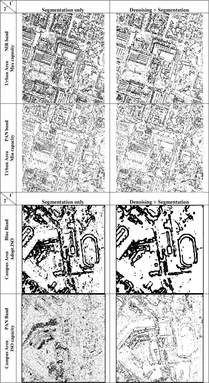
* 1 - Method combination;

2 - Area type, Band name, Hölder Exponent capacity

Visual qualitative assessment of obtained segmentation result images confirms said-above general resumes. As complementary quantitative assessments the Standard Deviation and Image Contrast to the best advantage fit for photogrammetric image segmentation estimation, and could be supplemented and compared with standard features of digital images visual quality in future studies.

These data allow concluding the following:

• -    The Multifractal pointwise Hölder exponent based segmentation of photogrammetric image fixed in a number of spectral ranges is performed.

• -    The segmentation results are estimated up to visual perception and qualitatively.

• -    As we can see, it should be experimented with different capacities and look at the result before you decide which one you choose: different capacities will often highlight different aspects of the image.

Good practical results give Preliminary Adoptive Wiener Denoising applied to the original images. So, it`s reasonable to study different de-noising approaches including Fractal de-noising methods, which should be applied to the image before the segmentation process begins.

Further development of the photogrammetric image segmentation may hold towards adding the preliminary image processing by means of de-noising methods, geometrical correction of spatial intensity distributions, image fusion methods for multispectral photogrammetric images and etc...

It`s also practical to study the post processing direction of object contours joining and elongation that had been suffered breaking during coarse segmentation.

Acknowledgment

The author sincerely and strongly felt thanks to Prof. Vladimir M. Korchinsky for the mere suggestion and supporting the research.