The rationale for the method of calculating the angles of arrival of short radio waves taking into account the influence of regular and random inhomogeneities of the ionosphere

radio wave enters the ionosphere φ (angle of incidence) and the angle at which radio wave comes out of the ionosphere φB are experienced random perturbations γ1 , γ2 (scattering parameter). These random perturbations have the same characteristics, they distribute by the normal law.

,

In order to determine a value of scattering parameter (in degree), we use the method that was presented in work of A.I. Agaryshev [3]. We choose on the Earth’s surface segments with length of ∆ and for rays with propagation length of Di , getting in the k-th segment, we calculate the mean values of elevation angles, arrival angles and reflection heights of radio waves θ_k, β_k, h_k respectively, and we can calculate the standard deviations of these averages σ . By changing the value of scattering parameter to match the measured and the calculated standard deviations allows us to determine the value of scattering parameter for the specific conditions. The characteristic scale of disturbances s at height of 100 km ≈ 100 m, when the height increases to 300 km the characteristic scale of disturbances increases to 100 km. The degree of the disturbance effect on the radio trajectory is defined by relation ∆χ/s , where ∆χ = ∆N/N – a disturbance of the electron concentration, it displays in percent, s – characteristic scale of disturbances. It was known that ∆χ ≈1% at height of 100 km and ∆χ ≈ 10% – at height of 300 km, therefore relation ∆χ/s at the height of 100 km is over 100 times in compared with the relation Δχ/ s at the height of 300 km.

The method of construction of trajectories HF radio waves is based on application of the modified Snell’s law for a thick layer of the ionosphere. For a thick layer Snell’s law is given by formula [4]:

n ⋅ R ⋅ sin( ϕ ) = n ₁ ⋅ R ₁ ⋅ sin( ϕ ₁ ) , (1)

where n, n₁ – refraction coefficients of environment at a level of “n” and “1”, R, R₁ – radius from the Earth’s center to the level “n” and “1”, φ and φ1 – angles between the path of radio wave and the radius R , R₁ . The electron density is defined in accordance with the ionospheric model [5].

According to Fig. 1 trajectory HF radio waves consists of three parts: 1) a direct path between the transmitter and lower boundary of the reflective layer, 2) a сurved path in the reflective layer, 3) a direct path between the lower boundary of this layer and the receiver. The method of construction of trajectory HF radio wave at path 2 is to divide it into equal segments, the length of these segments is substantially smaller than the total length of the curved path. Then the law (1) is applied sequentially to each of segments.

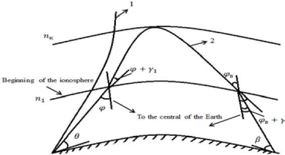
Fig. 1. The model of “beginning of the ionosphere”: 1 – refraction ray, 2 – reflection ray

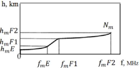
Fig. 2. The model of plasma frequencies for the ionospheric layers E, F1, F2 [5]

Then, a description of three-layer model of the ionosphere and mathematical expression of height dependence of the plasma frequency of ionospheric layers E, F1, F2 are given (Fig. 2). According to this model, the plasma frequencies are quadratic functions of height for layers E and F2 .

For the layer E: hmE = 110 km, semi-thickness ymE = 20 km, f pias ( h ) = f m E •

h-h

m

1 — -----------

I y m E J

.

When 110 ≤ h ≤ hmF 1 (layer F1 )

fp Os (h) = f m E • ( h • 0.225 + h m F 1 — 1.225 • h m E ) /( h m F 1 — h m E );

When hmF 1 < h <  hmF 2 (layer F2 ): f_plas ( h ) = f m F 2 •

^^^^^s

h

^— h m F ² ) y m ^{F 2 J}

A method for constructing trajectory HF radio wave

When taking into account the gradient of electronic concentration in horizontal direction of HF radio waves, the formula of refraction law as follows:

S ( R )

nk. R. s_m« _{P l} ) - n, - 1 . R, „. sinto - , ) = -£ ( — dS ,

,     dn where – the gradient of refractive index; dS – the element of trajectory radio wave.

B6

The right part of the equation (2) can be calculated approximately according to a formula:

f ^{S (} R k ) ^ n • dS «^n • ( S ( R ) - S ( R J) = ^ n • A S ,

J s ( R k - 1 ) d@        d0 ^x k ^{k 1}      60

where A S = S^(R i ) - S^(R o ) ^- a calculation step along trajectory.

For a small increment of central angle Δθ (Fig. 3), we have an approximate expression:

Ad ~ sin( AO )= d=- . Rk - 1

Where dx – an increment of distance by one moving step of radio waves in the ionosphere, Rk –1 – a radius between the central of the Earth and a starting point of k-th moving step.

In order to determine a value of refractive index n , we use a known formula:

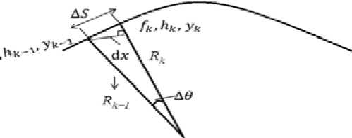
Fig. 3. Calculation of gradient of refractive index with an increment of central angle Δθ

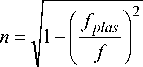
Where f, fplas – a carrier and a plasma frequencies respectively.

By using the three-layer model of the ionosphere and the expression (4), the value of refraction index can be defined through the critical frequency, the height of maximum ionization, the semithickness and a height of current point:

In the layer Е :

n ( h ) =

1 I ^f™^E I 1 I ^h - ^hm^E I

¹ - I             I ' ¹ - II

\ I f J L l Ут^Е J

In the layer F1 :

( f Л i /г-0 225 +/г Fl-1 225-/г E f mE          ^-5 ⁺ m       ^.^5 m

⁽⁾ ’H / П    V 1 - mE

In the layer F2 :

( f FlA ² Ih-h F2^

n ( h ) =

1 -I fmI • 1 -I h—hmI f           y F2

V f / V ym 7

With a very small value of 86, by taking into account the expression (3), we can calculate the gradient of refractive index as following:

dn_ , ^ = R k -Л n ( hdX ^{- n (} h ,) ] .                                       (5)

Where n ( h_{k –1}) and n ( h_k ) – the values of the refractive index at the beginning and the end of the k-th step of the movement of radio waves, corresponding to the heights hk –1 and hk .

For each movement step of radio waves, we calculate the values of critical frequencies of the ionospheric layers E and F2 (fmE, hmF2) and the height of maximum ionization hmF2. At the end of the dn movement step we find gradient of refraction index - by formula (5).

Then, by the expression of the Snell’s law (2) we can calculate the angle of incidence for a next movement step of radio wave:

nfc-i • R-i •sin( ^k-1) -     • AS sin( ^k) =---------------------б®---- nk • Rk

Radio wave is reflected from the ionosphere at the height where the angle of incidence equals to 90°.

A calculation program of arrival angles of HF radio waves

The program provides two modes of calculation: the first mode – calculate diurnal variation of arrival angles of considered mode of radio wave in a receiving point. The second mode – predict elevation angles and arrival angles of all modes of HF radio waves that are taken in a given area at a given specific time. Input data as follows: date, time, the average number of sunspot – the Wolf number (W) that corresponds to the given date, geographical coordinates of the transmitter and the receiver, the scattering intensity s that can be determined by method in work [3], a minimum and a maximum of elevation angle, step of angle Δθ , calculation step along trajectory radio wave ΔS .

By using the input data, block 1 determines the parameters of the ionosphere fmE, fmF2, M(3000) F2 that is close to a transmitter and a receiver using table-valued parameters of vertical sounding (VS) of the ionosphere, measured in days and hours of experimentation. Then, we define the peak height of the layer F2 of points of transmission and reception according to the formula developed in [3]:

h mF 2

7 M (3000)² - 1

- 176.

Unit 2 calculates the length of the route D and the azimuth of A radio link according to the specified geographical coordinates transmission and reception. Unit 3 implements calculations of angles of radiation and reception for each value of the angle of radiation. The values of the radiation angle changes from θmin to θmax in increments of ∆θ . The output from block 3 is a data array of angles of radiation and reception of radio waves received at the point of reception. In block 4, average values of angles of radiation and reception are calculated (n – number of hits). Fig. 5 shows the interface of the program. Unit 6 displays graphical and tabular results of calculations.

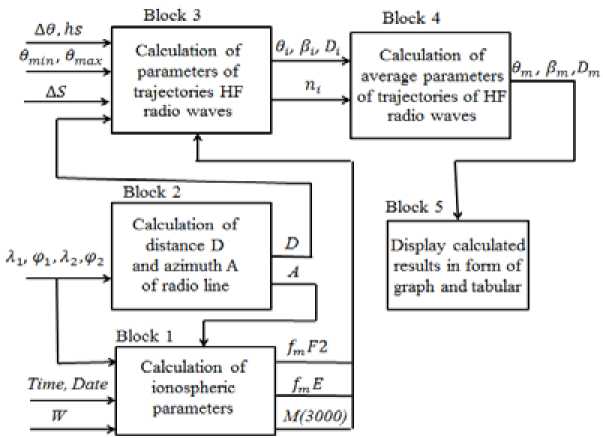
Fig. 4. A block-diagram of the program

Fig. 5. Interface of the prediction program of arrival angles HF radio waves [6]

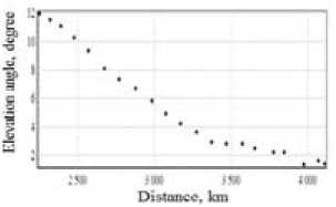
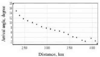
Fig. 6. Dependence of elevation angles and arrival angles on distance of mode 1F2 with f =18 MHz

Fig. 6 shows prediction results of elevation and arrival angles of HF radio waves in the form of graphs. Obviously, the elevation angles in this case are less than the arrival angles.

Comparisons with measured results

Examples of using the program for calculating arrival angles are presented below. On path Khabarovsk – Irkutsk the average values of measured data of arrival angles for moths in years [3] were used. We can see on Fig. 7 that, the calculated results (that equal to 8°) of method that is described in work [1] are less agreement with the experiments than the calculated results of presented method. Difference between calculated results of the proposed method and experiment data is caused by differences between prediction results of ionospheric parameters and actual parameters.

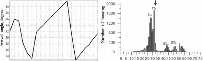
As the next example, predictions of arrival angles of HF radio by paths Moscow – Rostov-on-Don and Minsk – Rostov-on-Don are presented. The calculated results are compared with the experimental data of mode 1F2. The description of experiment were presented in [7]. The Wolf number was 72 in November, 90 in December by data in [8]. The calculated results from Fig. 8 have showed that, in the time interval from 5:00 to 6:00 MSK (Moscow standard time) the average value of arrival angles is 35°. The Agreement between the calculated results and experimental data of mode F20 (an ordinary component of mode F2 that is shown by the arrow) is good as shown in Fig. 8.

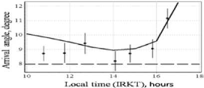
Fig. 7. Calculated results by method [1] (dashed curve), calculated results by proposed method (solid curve) and experimental results (points with confident limits) of dependence of arrival angles HF radio waves on local time in the middle of path Khabarovsk – Irkutsk in October

14 15 16 1" 18 19 20 21 22 23 24                      Arriviil angle, degree

MSK, hour

Fig. 8. The dependence of arrival angles of HF radio waves on time by path Moscow – Rostov-on-Don (left) and experimental distribution of arrival angles (right), 23.11.2013, 5:00–6:00 MSK f =4.996 МHz [7]

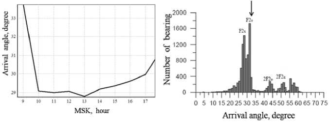
Fig. 9. Dependence of arrival angles of HF radio waves on time by path Moscow – Rostov-on-Don and experimental distribution of arrival angles, 23.11.2013, 9:00 – 10:00 MSK, f =9.996 MHz [7]

Fig. 9 shows that in the time interval from 9:00 to 10:00 MSK the angles of arrival HF radio vary in the range of 29 to 34° and the average value of arrival angles is 32°. These calculated results have a good agreement with measured results of mode F20 – the ordinary component of mode 1F2 that is presented in the same figure.

It notes that there was not observed mode 2F2 from prediction results in range of 9:00 to 10:00 MSK with transmitting frequency of 9.996 MHz and in range of 5:00 to 6 MSK with transmitting frequency of 4.996 MHz although by experimental data (Fig. 8 and 9, right) this mode was obtained. In order to explain this phenomenon, a maximum usable frequency of mode 2F2 – (MUF) 2F2 – 580 – was calculated for path Moscow – Rostov-on-Don by the method that is presented in work [3]. The calculated results of (MUF) 2F2 in 5:00 and 6:00 (MSK) are 3.4 and 3.95 MHz respectively, at 9:00 and 10:00 AM (MSK) – (MUF) 2F2 are 7.45 and 8.3 MHz respectively. These calculated results show that, theoretically, in the range of 5:00 to 6:00 MSK with transmitting frequency 4.996 MHz modes 2F2 can not be observed and in the range of 9:00 to 10:00 MSK with transmitting frequency 9.996 MHz modes 2F2 also can’t be observed. In spite of this, practically, propagations of HF radio with transmitting frequency higher MUF 2F2 are possible (as were shown in Fig. 8, 9) by reasons of influences of the random inhomogeneous ionosphere. There are two types of random inhomogeneous ionosphere: 1) the random small-scale inhomogeneities (characteristic size < 1 km) that is located lower reflected layer. 2) the random large-scale inhomogeneities (characteristic size >100 km) that is related with traveling ionospheric disturbances (TIDs). In a work [3], the method “equal MUF” is presented that has given the same data of calculation MUF 2F2.

From the graph in Fig. 10, we can note that the average value of arrival angles of mode F2 in the range from 13:00 to 14:00 MSK is 33°. These results are consistent with measured results of the ordinary component of mode 1F2.

From graph in Fig. 11 (left), the average value of arrival angles from 14:00 to 15:00 MSK can be determined and it equals to 23.5°. This calculated result is more than experimental data on 2°. This deviation is quite acceptable with considering of reliability of determining of input data.

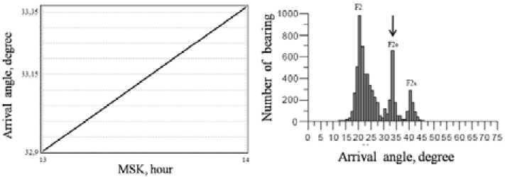
Fig. 10. Variations of arrival angles of HF radio waves by path Moscow – Rostov-on-Don and experimental distribution of arrival angles, 09.12.2013, 13:00–14:00 MSK, f=14.996 MHz [7]

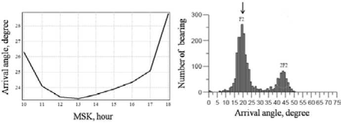
Fig. 11. Variations of arrival angles of HF radio waves by path Minsk – Rostov-on-Don and experimental distribution of arrival angles, 01.12.2013, 14:00–15:00 MSK, f =11.730 MHz [7]

Optimization of antenna diagram

In order to design HF antennas, it is very important to give the angles of arrival of HF radio waves. We can use the proposed program for calculating arrival angles. Let us give an example of design of a horizontal rhombic antenna for path from Khabarovsk to Irkutsk with operating frequency 16.8 MHz. The radiation pattern in the vertical plane of horizontal rhombic antenna is given by an expression [9]:

F ^{( 6 )} = 1---- ■⁸ /4 ' sin² 1 “Г р ^{[ 1} - s ⁱⁿ⁽ ^ ) ' ^c o ^{s( 6} m ^{) ]}f ' ^sin( k ' H P ' ^{sin( 6} m ) .

1 - ^sin( ф ⁾ • ^cos( 9 m )      [ 2                        J

Where θm – an arrival angle HF radio wave, φ – a half of obtuse angle of rhombic, lp – a length of sides of rhombic, H_П – a suspension height above ground of antenna.

Using the proposed program, we can determine the radiation pattern for the average angle of arrival on path Khabarovsk-Irkutsk with an operating frequency of 16.8 MHz. In order to solve this problem, firstly, a prediction of arrival angle HF radio on route Khabarovsk – Irkutsk is carried out. Further, by using the calculation results, we can determine the average value of the arrival angles of radio waves in year. The calculated results were shown in Table.

Following the table, the average value of arrival angles of radio waves equals to 11.2° in year. From the handbook [9], we can choose the rhombic antenna RH(65/4)1 with parameters φ = 65°, l = 4 λ 0 , H = λ ₀ with a maximum of the main lobe of the radiation pattern, which corresponds to the calculated arrival angle of mode 1F2 of HF radio waves, the minimum of radiation pattern corresponds to arrival angles of mode 2F2 (Fig. 12).

Conclusions. This article successfully solved the problem of analysis of using the proposed program to solve practical problem, including:

Table. The average values of arrival angles HF (in deg) waves radio by path Khabarovsk – Irkutsk

Months	January	February	March	April	May	June
β cp	10.2	10	10.5	11	13.7	13. 2
Months	July	August	September	October	XT     к November	December
β	13.2	12.7	11.3	9.7	9.4	9.0

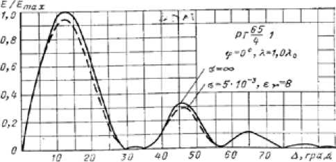
Fig. 12. Radiation pattern in the vertical plane of antenna RH (65/4)1 [9]

• 1)    Developing the method and building a program to calculate the angles of arrival HF radio waves. The method based on application of modified Snell’s law with considering the influence of gradient of refractive index on trajectories HF radio waves in the horizontally inhomogeneous scattering ionosphere.

• 2)    The comparisons with measured results by paths Khabarovsk – Irkutsk, Moscow – Rostov-on-Don, Minsk – Rostov-on-Don were carried out. As a result, our calculation agrees much better with measured data, compared to calculations from other methods based on the horizontal homogeneous ionosphere.

• 3)    Showing that the proposed program allows designing radiation pattern of HF antenna with the main lobe that corresponds to mode 1F2 and the minimum corresponds to mode 2F2.

The causes of deviations between the calculation results of arrival angles of HF radio waves and the measured results are obvious. The first deviation can be reduced by taking into account the extraordinary components of radio waves, the second deviation is relates to using a more efficient method for calculating MUF 2F2 that was known as reception of hops with equal MUF [3]. In our future works, we will work on improving the performances of the program and the proposed method to reduce the deviations.