The Study of Slow Manifolds in the Lorenz-Haken Model Using Differential Geometry

The existence of invariant manifolds in singularly perturbed systems where the flow trajectories move slowly has been established in previous works [1, 2]. Different methods have been developed to find the analytical equations of these slow manifolds, such as the geometric singular perturbation technique [3, 4]. However, this technique fails to provide the slow manifold equation for non-singularly perturbed systems like the Lorenz-Haken (L-H) model.

A single mode unidirectional ring laser that contains a homogeneously-broadened, two-level medium, known as the Lorenz-Haken model, serves as the simplest laser model. Haken [5] discovered the equivalence between the Lorenz model that describes fluid turbulence [6] and the equations of a homogeneously-broadened, single-mode laser in 1975. Under suitable conditions, such a laser system becomes unstable, characterized by respective values of decay rate (bad cavity condition) and level of excitation (second laser threshold). Numerical integration of the Lorenz-Haken model indicates that the system undergoes a transition from a stable continuous wave output to a regular pulsing state. However, it can also develop irregular pulsations (chaotic solutions), whose nature Haken explained. For over thirty years, finding the pulsing solutions of the single-mode laser equations involved numerical integration. Bougoffa and Bouggouffa [7, 8, 9] proposed an analytical approach using Adomian decomposition to solve the Lorenz system.

A novel method for finding the implicit equation of the slow manifold, applicable to any dynamical system in any dimension, singularly disturbed or not, has recently been developed [10, 11]. It is called the flow curvature method. The FitzHugh-Nagumo model, the Brusselator model, the Van der Pol model, the Chua's model, the Lorenz model, and the Rikitake model have all been successfully used the flow curvature approach. The generalized Lorenz-Krishnamurthy model and conservative generalized Lorenz-Krishnamurthy model's slow invariant manifold analytical implicit equation was created in [12]. This technique was utilized in [13] to build the heartbeat model's slow invariant manifold.

Researchers have studied a variety of slow-fast dynamical models that are helpful in science and engineering [14, 15, 16].

The major research objective is to find the slow invariant manifold analytical equation of the L-H model. In order to get the analytical implicit equation of the slow invariant manifold for the three-dimensional L-H model, we employ the flow curvature approach in this study. There are numerous methods available to determine the slow manifold analytical implicit equation of the model we present. Slow eigenvectors [17], an iterative approach [18] have all been used in earlier slow manifold’s calculations for the L-H model. No dimensional constraint or asymptotic expansion is necessary for our recommended approach. First, using the flow curvature approach, we identify the slow manifold analytical implicit equation of the L-H model and then we prove the invariance of the slow manifold of the L-H model using the Darboux theory. To simulate the L-H model, we utilize the program MATHEMATICA.

The remainder of this article is divided into the following sections. Section 2 introduces the nonlinear optical slow-fast L-H model. The flow curvature approach based on differential geometry is described in Section 3, along with the Darboux theorem that proves the slow manifold of a dynamical system is invariant. We present the analytical equation of the slow manifold for the L-H model in Section 4. Concluding observations and additional commentary on the study's findings are provided in Section 5 of this report.

2.    Lorenz-Haken Model

The starting point of the model is the Maxwell-Bloch equations in the single mode approximation, which describes the behavior of a unidirectional ring laser containing a homogeneously broadened medium. A semi-classical approach is used to derive the equations of motion by considering the resonant field inside the laser cavity as a macroscopic variable interacting with a two-level system. The model assumes exact resonance between the atomic line and the cavity mode and makes some appropriate approximations. After these approximations, three nonlinear differential equations are obtained, which describe the behavior of the field, polarization, and population inversion of the medium. This set of equations is commonly referred to as the L-H model. The standard L-H model's slow-fast system is as follows:

dx dt dy dt dz dt

• -    k ( x + 2 cy ) ,

(1) - y + xz ,

• -    d (1 + xy + z),

3.    The Flow Curvature Technique

• 3.1.    The Implicit Analytical Equation of the Slow Manifold of the Dynamical System

where the electric field in the laser cavity is denoted by x(t) with a decay constant к, the polarization of this field is represented by y(t) , and the population difference is indicated by z(t) with a decay constant d . Both к and d are normalized with respect to the polarization relaxation rate, and 2C is the pump rate necessary to achieve the lasing effect. In order to obtain the steady-state solution of the system, all time derivatives are set to zero. However, under certain circumstances, the steady-state solution becomes unstable. Linear stability analysis can be used to determine the boundary regime where the equations become unstable.

In this section, we will explore the use of differential geometry in analyzing the dynamical model. The technique involves studying the curvature of the trajectory curve, which allows us to obtain the flow curvature manifold. For any n -dimensional dynamical model, there exists a (n — 1) dimensional flow curvature manifold which contains information about the flow with the maximum curvature.

Understanding the stability and behavior of a slow-fast system depends on the invariant manifold. A sluggish manifold's equation can be found using the traditional approach of geometric perturbation. It doesn't need eigenvectors or asymptotic expansions like the flow curvature approach requires. It is also applicable to all dynamical systems, singularly disturbed or not.

Lemma 3.1 The equation of the flow curvature manifold of a dynamical system represents the set of points where the curvature of the system's flow vanishes.

0 ( W ) = det W , W , W ,

_{,   , W} ( n )

= 0

Proof See [10]

Lemma 3.2 The analytical equation of the slow manifold can be obtained directly from the implicit equation of the flow curvature manifold.

Proof See [10]

• 3.2.    Darboux Invariance Theorem

  According to [19], G. Darboux originally proposed the idea of the invariant manifold in 1878. In this study, we represent the trajectories of the dynamical system (1) as the motion of a point in a three-dimensional space, where the point's coordinates are denoted as W = (x, y, z) and its velocity vector as V = (x, y, z) .

4.    Using the Flow Curvature Method to Analyze Dynamic L-H Model

Lemma 3.3 Assume that ^ W ) = d_et ^ W , W , W ,..., W^{( n} ) j ₌ 0 is a continuously differentiable function of the first order that represents a slow manifold of the dynamical system (1). Then, this manifold is invariant concerning the flow of (1) if there exists a continuously differentiable function, referred to as cofactor R ( W ), which satisfies the following equation:

£y 0(W) = R (W )0(W), with the following Lie derivative:

Cy 0 ( W ) = V -V0 = d 0/ dt

Proof See [10]

The flow curvature method is a technique that considers the trajectory curves of a dynamical system, whether singularly perturbed or not, as curves in the Euclidean space. In this study, The flow curvature approach is used to the slow-fast dynamical system described by model (1).

To perform numerical simulations, we utilize the parameter values provided in Table 1, and let, a measure of the state variables' range associated with model (1) as follows:

[x min , x max ] = [-15, 15];

[ymin , ymax ] = [-15, 15];

[zmin , zmax ] = [-15, 15];

Table 1. For the numerical calculations, typical model (1) parameter values..

Parameters	k	c	d
Values	3	9.2	0.1

By arranging the dynamic system's right-hand side components (1), that is,

- k ( x + 2 cy ) = 0 ,

- y + xz = 0,                                                   ⁽²⁾

- d (1 + xy + z ) = 0,

For the null-clines of the model (1), we get the following graphs.

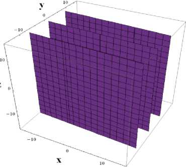
(a)

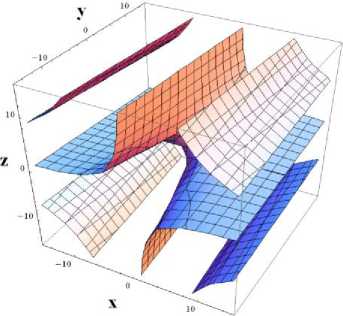
(b)

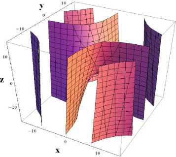
(c)

Fig. 1. (a) The Nullcline of the first equation of model (1), (b) The Nullcline of the second equation of model (1), and (c) The Nullcline of the third equation of model (1).

As a result, after solving the system of equations (2), we get the fixed points as follows:

x1 = -4.17, y1 = 0.23, z1 = -0.05

x2 = 0, y2 = 0, z2 = -1

x3 = 4.17, y3 = -0.23, z3 = -0.05

The model's Jacobian matrix at the fixed point is as follows:

' - 3 - 55.2 0 ⁴

z - 1 x ^- 0.1 y - 0.1 x - 0.1 ^

The following formulae are used to express the eigenvalues of the aforementioned Jacobian matrix that correspond to model (1) at the fixed points:

{-4.18477, 0.0423868 - 1.57891 i, 0.0423868 + 1.57891 i}

{-9.49667, -0.1, 5.49667}

{-4.18477, 0.0423868 - 1.57891 i, 0.0423868 + 1.57891 i}

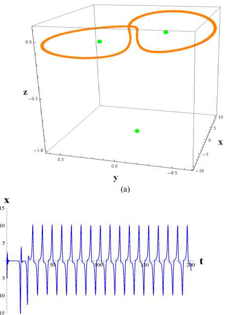
We employ the fourth order Runge-Kutta approach to resolve the flow model (1), where we consider as a starting point. The phase plot's three-dimensional graphical behavior, with a t range of 0 to 1000, is shown in Fig. 2 (a). The three-dimensional parametric plot of this, where t is a value between 50 and 1000, is computed using mathematics. The green point in Fig. 2 (a) denotes the model's fixed points.

y

(b)

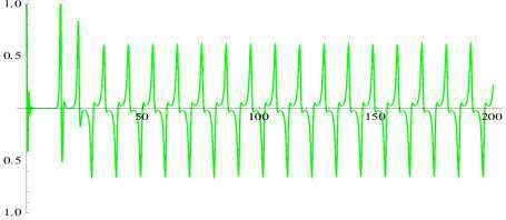
t

z

(c)

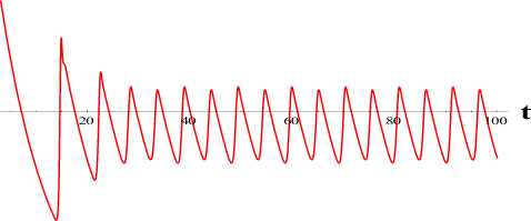
(d)

Fig. 2. (a) The Phase plane result and three fixed points; (b) The Time series solution of x; (c) The Time series solution of y; and (d) The Time series solution of z.

We create three-dimensional parameter charts using the numerical simulation of model (1), where spans from 0 to 1000. Fig. 2(b) shows the periodic solution behavior of the variables x,y, and z, whereas Fig. 2(c) shows the periodic solution behavior of the variables у and z.

We now compute the acceleration vector and velocity vector first in line with the FCM.

The following is the model (1)'s velocity vector.

V1={-3 (x + 18.4 y), -y + x z, -0.1 (1 + x y + z)}

The acceleration vector may now be expressed as follows:

• V ₂={-55.2 (-0.163043 x - 4. y + 1. x z), -0.1 (1. x - 10. y + 1. x² y + 41. x z + 552. y z), 5.52 (0.00181159 + 0.0742754 x y + 1. y² + 0.00181159 z - 0.0181159 x² z)}

The over-acceleration (jerk) vector may thus be expressed as follows.

• V ₃={0. + 165.6 (-0.163043 x - 4. y + 1. x z) + 5.52 (1. x - 10. y + 1. x² y + 41. x z + 552. y z), 0.6 (x + 18.4 y) (1 + x y + z) - 55.2 z (-0.163043 x - 4. y + 1. x z) + 5.52 x (0.00181159 + 0.0742754 x y + 1. y² + 0.00181159 z - 0.0181159 x² z) + 0.1 (1. x - 10. y + 1. x² y + 41. x z + 552. y z), 0. + 0.6 (x + 18.4 y) (-y + x z) + 5.52 y (-0.163043 x - 4. y + 1. x z) -0.552 (0.00181159 + 0.0742754 x y + 1. y² + 0.00181159 z - 0.0181159 x² z) + 0.01 x (1. x - 10. y + 1. x² y + 41. x z + 552. y z)}

The slow manifold function may now be stated as follows.

Θ (x, y,z) = 0.003 (-134.4 x² + 1. x⁴ - 6262.8 x y - 244.8 x³ y + 2. x⁵ y - 93630.2 y² - 9562.8 x² y² + 49.6 x⁴ y²

+ 1. x⁶ y² - 95661.6 x y³ + 4140. x³ y³ + 2.31296*10 ^{- 15} x⁵ y³ + 481432. y⁴ + 135085. x² y⁴+ 1.68197*10⁶ x y⁵ - 1247.4 x² z + 71. x⁴ z - 32648.4 x y z + 3636.6 x³ y z - 9. x⁵ y z - 742650. y² z + 85946.4 x² y² z + 1104. x⁴ y² z + 125944. x y³ z + 30470.4 x³ y³ z - 1.06525*10⁷ y⁴ z - 12153. x² z² + 496. x⁴ z² + 10. x⁶ z² - 229522. x y z² + 36432. x³ y z² + 7.40149*10 ^{- 14} x⁵ y z² - 6.25557*10⁶ y² z²

• +    1.06646*10⁶ x² y² z² + 1.68197*10⁷ x y³ z² - 112608. x² z³ + 11040. x⁴ z³ - 203136. x y z³ + 304704. x³ y z³

• -    5.60655*10⁶ y² z³ - 101568. x² z⁴)

The flow curvature manifold of the model (1) now provides the slow manifold's equation.

Θ ( x , y , z ) = 0                                                       (3)

Fig. 3 (a) depicts the slow manifold of the model (1) visually. Fig.3(b) displays a visual representation of the phase diagram and slow manifold.

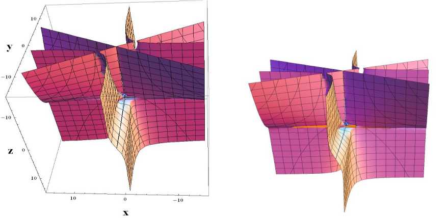
(a)

(b)

Fig. 3 (a) The model (1)'s flow curvature manifold; (b) the phase diagram and the flow curvature manifold together.

We begin by determining the flow curvature manifold’s perpendicular vector ∇Θ . The Darboux theory and this normal vector ∇Θ may then be used to find the Lie derivative ^v Θ . It is possible to express the normal vector ∇Θ as:

• {0 .003 (-268.8 x + 4. x³ - 6262.8 y - 734.4 x² y + 10. x⁴ y - 19125.6 x y² + 198.4 x³ y² + 6. x⁵ y² - 95661.6 y³ + 12420. x² y³ + 1.15648*10^-14 x⁴ y³ + 270171. x y⁴ + 1.68197*10⁶ y⁵ - 2494.8 x z + 284. x³ z - 32648.4 y z + 10909.8 x² y z - 45. x⁴ y z + 171893. x y² z + 4416. x³ y² z + 125944. y³ z + 91411.2 x² y³ z - 24306. x z² +

• 1984.    x² z² + 60. x⁵ z² - 229522. y z² + 109296. x² y z² + 3.70074*10^-13 x⁵ y z² + 2.13293*10⁶ x y² z² + 1.68197*10⁷ y³ z² - 225216. x z³ + 44160. x³ z³ - 203136. y z³ + 914112. x² y z³ - 203136. x z⁴), 0.003 (-6262.8 x - 244.8 x³ + 2. x⁵ - 187260. y - 19125.6 x² y + 99.2 x⁴ y + 2. x⁶ y - 286985. x y² + 12420. x³ y² + 6.93889*10^-15 x⁵ y² + 1.92573*10⁶ y³ + 540342. x² y³ + 8.40983*10⁶ x y⁴ - 32648.4 x z + 3636.6 x³ z -

• 9.    x⁵ z - 1.4853*10⁶ y z + 171893. x² y z + 2208. x⁴ y z + 377833. x y² z + 91411.2 x³ y² z - 4.26098*10⁷ y³ z -

  229522. x z² + 36432. x³ z² + 7.40149*10^-14 x⁵ z² - 1.25111*10⁷ y z² + 2.13293*10⁶ x² y z² +

  • 5. 0459*10⁷ x y² z² - 203136. x z³ + 304704. x³ z³ - 1.12131*10⁷ y z³),

    0.003 (-1247.4 x² + 71. x⁴ - 32648.4 x y + 3636.6 x³ y - 9. x⁵ y - 742650. y² + 85946.4 x² y² +

    • 1104.    x⁴ y² + 125944. x y³ + 30470.4 x³ y³ - 1.06525*10⁷ y⁴ - 24306. x² z + 992. x⁴ z + 20. x⁶ z -

    • 459043.    x y z + 72864. x³ y z + 1.4803*10^-13 x⁵ y z - 1.25111*10⁷ y² z + 2.13293*10⁶ x² y² z + 3.36393*10⁷ x y³ z - 337824. x² z² + 33120. x⁴ z² - 609408. x y z² + 914112. x³ y z² - 1.68197*10⁷ y² z² - 406272. x² z³)}

Now, the sluggish manifold's Lie derivative ^vΘ may be expressed as

• -2.35922*10^-17 (-1.18404*10¹⁷ x² + 2.42876*10¹⁵ x⁴ - 5.48746*10¹⁸ x y - 2.52831*10¹⁷ x³ y + 4.85753*10¹⁵ x⁵ y - 7.72159*10¹⁹ y² - 1.42053*10¹⁹ x² y² + 2.18774*10¹⁷ x⁴ y² + 2.42876*10¹⁵ x⁶ y² -2.15076*10²⁰ x y³ + 9.19031*10¹⁸ x³ y³ + 5.61541*10¹⁶ x⁵ y³ - 5.62054*10²⁰ y⁴ + 2.60556*10²⁰ x² y⁴ + 3.87463*10¹⁷ x⁴ y⁴ + 3.47198*10²¹ x y⁵ + 1.18062*10²² y⁶ - 4.80277*10¹⁷ x² z + 1.52987*10¹⁷ x⁴ z -1.65582*10¹⁹ x y z + 9.71352*10¹⁸ x³ y z - 1.84256*10¹⁶ x⁵ y z - 5.86575*10²⁰ y² z + 2.22882*10²⁰ x² y² z + 1.01077*10¹⁸ x⁴ y² z + 1. x⁶ y² z + 1.32804*10^²¹ x y³ z + 3.62924*10¹⁹ x³ y³ z - 4.6697*10²¹ y⁴ z -77101.2 x² y⁴ z - 9.72556*10¹⁸ x² z² + 7.28197*10¹⁷ x⁴ z² + 2.42876*10¹⁶ x⁶ z² - 1.12069*10²⁰ x y z² + 4.665*10¹⁹ x³ y z² + 5.61541*10¹⁷ x⁵ y z² - 3.57497*10²¹ y² z² + 1.8234*10²¹ x² y² z² + 2597.65 x⁴ y² z² + 3.34365*10²² x y³ z² + 1.18062*10²³ y⁴ z² - 6.61916*10¹⁹ x² z³ + 1.26347*10¹⁹ x⁴ z³ - 9.41176 x⁶ z³ -1.00999*10²⁰ x y z³+ 4.32667*10^20 x³ y z³ - 3.06561*10²¹ y² z³ + 1.23362*10⁶ x²y² z³ - 5.68279*10¹⁹ x² z⁴ -3.87463*10¹⁹ x⁴ z⁴)

5.    Conclusion

The equation £p0 = 0 , which denotes that The flow curvature manifold's rate of change 0 ( x , y ) = 0 , is graphically depicted in Figure 4(a). The phase diagram and the equation for the slow manifold's invariance are shown visually in Figure 4(b).

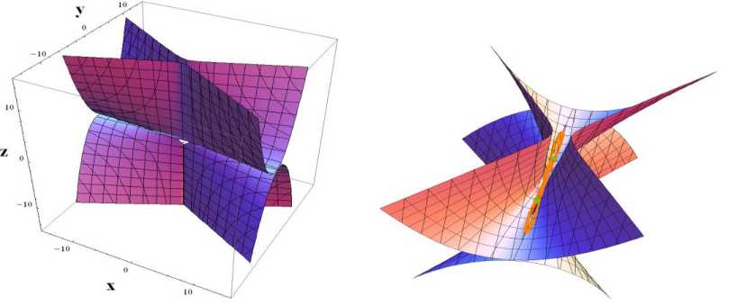
(a)                                                                      (b)

Fig. 4. The slow manifold's invariance equation is shown in (a), and the phase diagram and slow manifold's invariance equation are shown in (b).

This work investigated the L-H model using the flow curvature approach, a recently developed technique that uses differential geometry to the analysis of dynamical systems. Analytical calculations were made to determine the flow curvature manifold, which represents the temporal derivatives of the velocity vector field and offers details on the dynamics of the system. The L-H model is a nonlinear optical slow-fast dynamical system, and in this study, the flow curvature approach was used to evaluate the L-H Model’s slow invariant manifold. With the use of the Explicit Runge-Kutta technique, the analytical equation for the slow invariant manifold was discovered. The slow manifold was shown to be invariant using the Darboux invariance theorem, which showed strong agreement with the flow curvature manifold. For the first time, we specifically investigated the slow manifold of the three-dimensional L-H model using the flow curvature approach, and this research improves the field relative to earlier relevant work.