The use of the inverse transformation method for time series analysis

Introduction. For the specialists involved in data analysis, in most cases prediction may be said to be the main goal and task. Modern methods of statistical forecasting are often able to predict almost any possible indicators with high accuracy [1].

Forecasting is a system of scientifically based ideas about the possible conditions of an object in the future and alternative ways of its development [2]. There are no universal prediction methods for all occasions. Any practical forecasting problem can be satisfactorily solved only by a limited number of methods [3]. The choice of a forecasting method and its effectiveness depend on many conditions: the purpose of the forecast, the period of its lead prediction, the level of detailing and the availability of initial information [4]. The most commonly used forecasting method is mathematical modeling. A mathematical model is an approximate description of a specific process or phenomenon of the external world, expressed using a mathematical apparatus [5].

The components of the time series. Commonly, when studying a time (dynamic) series, it is depicted in the form of the following mathematical model: ^^

Yt = Y + Et where Yt – time series value; Yt – systematic (deterministic) component of the time series; Et – random component of the time series [6].

The systematic component of the time series Y t is a result of the influence of constantly acting factors on the process being analyzed. Two main systematic components of the time series can be distinguished:

• 1.    The trend of the time series.

• 2.    The cyclic oscillations of the time series.

A trend is a general pattern of change in the indicators of the time series, stable and observed over a long period of time. A trend is described using some function, usually monotonic. This function is called 'trend function', or simply “trend” [7].

Among the factors that form the cyclical oscillations of the series, in turn, two components can be distinguished:

• 1)    seasonality;

• 2)    cyclicity.

Seasonality is a result of the influence of factors acting at a predetermined periodicity. These are regular fluc- tuations that are periodic in nature ending within a year. The cyclic component is a nonrandom function that describes long (more than a year) periods of rise and fall [8; 9]

The random component of the time series E t is the component of the time series remaining after the allocation of systematic components. It reflects the effects of numerous random factors; it is a random, irregular component.

Random variables are diverse in nature and origin, although the distribution law can be written in a uniform universal form, namely, in the form of a distribution function that is equally suitable for discrete and continuous random variables [10].

Inverse Transformation Method. For forecasting purposes, as well as simulation, one may need a method for generating the random component of a time series. For this purpose, we use the inverse transformation method.

Let the random variable X have the distribution function F ( x ). We assume that F ^–1( x ) is the inverse function of F ( x ). Then the algorithm for generating the random variable X with the distribution function F ( x ) will be the following:

• 1.    Generate the value U having the uniform distribution over the interval (0;1);

• 2.    Return X = F ^–1( U ).

Fig. 2 depicts this algorithm graphically; the random variable corresponding to this distribution function can take either positive or negative values; it depends on the specific value of U . In Fig. 1, the random number U 1 gives the positive value of the random variable X 1 as a result, while the random number U 2 gives the negative value of the random variable X 2 as a result [11].

Estimating the distribution function of a random variable. Let us consider the time series as a sequence x ₁, x ₂, …, x_n of independent and equally distributed, according to a certain law, random variables; this sequence is called the sample of volume n. Each x_t ( t = 1, 2, ..., n ) is called variation. Having the sample, we do not have information about the form of the distribution function F ( x ). It is required to construct an estimate (approximation) for this unknown function.

The most preferred estimate of the function F ( x ) will be the empirical distribution function F n ( x ).

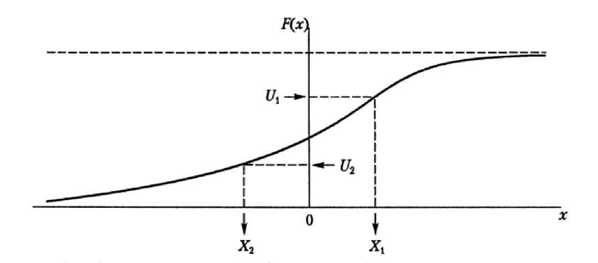
Fig. 1. Using the Inverse Transformation Method to generate a random variable

Рис. 1. Использование метода обратного преобразования для генерирования случайной величины

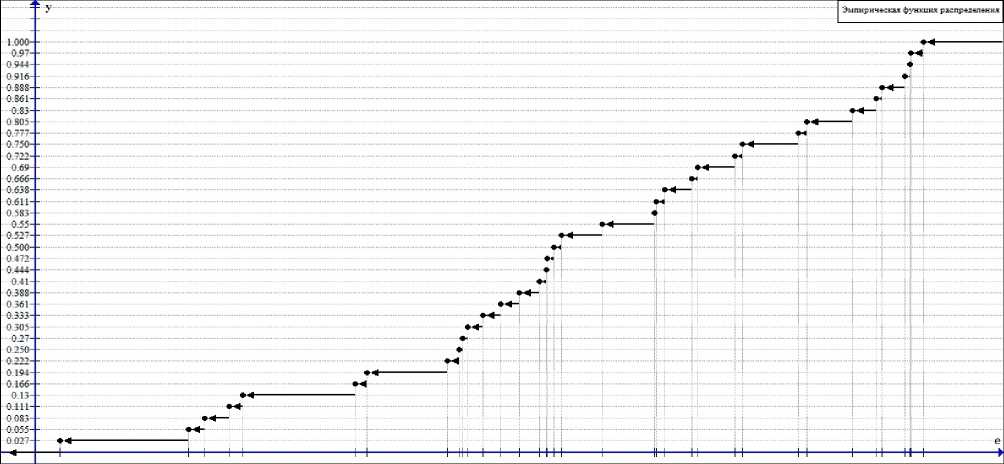
Fig. 2. Graph of the empirical distribution function F n ( e )

Рис. 2. График эмпирическая функция распределения F_n ( e )

The empirical distribution function (sampling distribution function) is the function F n ( x ), which determines the relative frequency of the event X < x for each x value, i. e.

и

Fn (х) = n^, n where nx – the number of xt values, less than x; n – sample size.

With a sufficiently large sample size, the functions F n ( x ) and F ( x ) = P ( X < x ) differ insignificantly from each other.

The difference between the empirical distribution function and the theoretical one is that the theoretical distribution function determines the probability of the event

X, and the empirical function determines the relative frequency of the same event [12].

The empirical distribution function has all the properties of the integral distribution function:

• 1)    the values of the empirical distribution function belong to the interval [0; 1];

• 2)    F n ( x ) is non-decreasing function;

• 3)    F_n ( х ) = 0 at х <  х min , if X min is the smallest variation;

F_n ( х ) = 1 at х >  х _min , if X _min is the largest variation [6].

However, to use the inverse transformation method, it is convenient to have a continuous distribution function; therefore, it is necessary to interpolate the obtained empirical function.

Building a predicted model. We give an example of using the inverse transformation method when constructing a predicted model. As the initial data, we use the average monthly indicators of power consumption in the Krasnoyarsk Territory for 3 years from January 2009 to December 2011 [13].

Using some regression model, the forecast values of the time series were calculated. Actual Y t and predicted Y_t values of the time series are presented in tab. 1

We build the empirical distribution function of the values of the deviations e_t of the predicted values Y_t from the actual values Y t of the time series e t = Y t - Y t . To do this, it is necessary to rank the sample { e t }, thus obtaining the sample { e ( _t ) = { e ₍₁₎ <  e (₂) < ... <  e ( n ) } (tab. 2).

Since the frequency of each variation equals 1, the empirical function will have the following form:

	0, ...;	e e	[-” ’ e (1) ) ;
F n ( е ) = ^	t_ n ’	e e	[ e ( t ) , e ( t + 1) ) ;	t = 0’1’..	., n
	...; 1’	e e	[ e ( n ) ’ 'Z 1 .

The graph of the function F n ( e ) is shown in fig. 2.

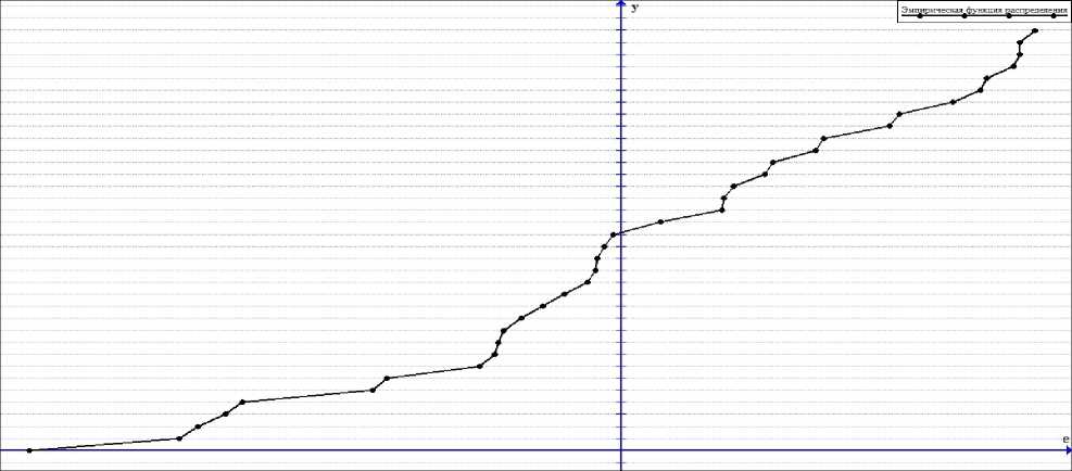
The obtained empirical function F n ( e ) has a discrete form. We use piecewise linear interpolation to obtain the continuous distribution function of the random variable F_n ^* ( e ). To do this, we use the equation of a straight line passing through two points:

I y? - y IУ = (x - x1) xl -------- 1 + У1.

I x 2 ^{- x} 1 )

The continuous distribution function of the random variable F_n ^* ( e ) will have the following form:

' 0,

F n ( e ) = {

^{( e} ' - ^e ( t ) )

¹ 1 ( n - 1 ) 1+ t - 1 , _v ^e ( t + 1) ^{- e} ( t ) ) ^{n - 1}

1,

^e ^ I ^z , ^e (1) ) ;

^{e e}f e ( t ) , e ( t + 1) ) ; t = 0,¹,..., n ;

e e[ e ( n ) , +“ ) .

Actual Y_t and predicted Y_t values of the time series

Table1

t	Y t	Y t	t	Y t	Y t	t	Y t	^^ Y t	t	Y t	^^ Y t
1	51.0123	53.09764	11	35.5809	43.42324	21	37.8690	44.58914	31	17.1468	15.15964
2	38.2345	38.37535	12	53.2584	54.26158	22	63.4957	57.61664	32	20.8548	21.45395
3	40.0023	35.24303	13	52.3887	52.69219	23	72.9843	72.28322	33	29.3791	31.55531
4	25.1288	32.13879	14	39.9125	41.30390	24	88.0214	83.09426	34	51.1710	44.09931
5	22.9338	27.08163	15	39.2113	32.14284	25	82.6095	79.01463	35	61.5869	59.79590
6	27.0146	20.64426	16	31.3420	24.38189	26	62.7282	63.15378	36	71.2594	73.02318
7	25.1154	17.77792	17	26.0102	19.52312	27	50.0250	48.20592
8	16.6987	19.20278	18	20.5578	17.87433	28	29.6211	34.02474
9	27.3114	23.86244	19	12.1214	22,62140	29	22.2954	22.75450
10	29.2400	31.48983	20	24.9374	32.44863	30	17.8092	15.25792

Range of Values e _t and e _{( t )}

Table 2

t	et	e ( t )	t	et	e ( t )	t	et	e ( t )	t	et	e ( t )
1	–2.085	–10.500	11	–7.842	–2,085	21	–6.720	1.791	31	1.987	6.370
2	–0.141	–7.842	12	–1.003	–1.764	22	5.879	1.819	32	–0.599	6.487
3	4.759	–7.511	13	–0.303	–1.391	23	0.701	1.987	33	–2.176	6.960
4	–7.010	–7.010	14	–1.391	–1.003	24	4.927	2.551	34	7.072	7.068
5	–4.148	–6.720	15	7.068	–0.599	25	3.595	2.683	35	1.791	7.072
6	6.370	–4.404	16	6.960	–0.459	26	–0.426	3.449	36	–1.764	7.337
7	7.337	–4.148	17	6.487	–0.426	27	1.819	3.595
8	–2.504	–2.504	18	2.683	–0.303	28	–4.404	4.759
9	3.449	–2.250	19	–10.500	–0.141	29	–0.459	4.927
10	–2.250	–2.176	20	–7.511	0.701	30	2.551	5.879

The graph of the function F ₃ ^* ₆ ( e ) is shown in fig. 3.

Evaluating the predicted model. For further analysis of this method, let us consider several forecast models [14]:

• 1.    We take the value Y_t of the time series as a completely deterministic process, to carry out the forecast we use the values Y_t calculated using the regression model;

• 2.    The value Y_t of the time series will be taken as a random variable for which we construct the distribution function F n ( e ) and calculate the predicted values Y, ;

• 3.    We will take the value Y_t of the time series as a set of values Y_t calculated using the regression model and the random component e t , for which we construct the distribution function F_n ^* ( e ) and calculate the predicted values e .

Let us make the operational prediction of energy consumption levels. For this purpose, we exclude from consideration the last 5 observations from the sample and we calculate new estimates of the parameters of the regression model, as well as the new distribution functions F3*1(x) and F3*1(e).

We apply the inverse transformation algorithm to the obtained functions F ₃ ^* ₁ ( x ) and F ₃ ^* ₁ ( e ). To this end, we generate the sample { u t } of random numbers having a uniform distribution in the interval [0; 1], and return Yt = F ₃*f1 ( u_t ) and e ' t = F ₃*f1 ( u_t ). The calculation results are presented in tab. 3.

When considering the obtained results, it is clear that the sum Y_t + e , is closer to the actual data than the predicted values calculated using the regression model. Thus, the predicted values smoothed out the predicted error to an extent (fig. 4).

As a criterion for assessing the quality of the model, we determine the value of the average approximation error, which is calculated using the formula [15]:

n

А = ¹ X n t = 1

(y -Y ) ( act pr )

Y .

act

■ 100%,

where Y pr – predicted value of time series; Y act – actual value of time series; n – size of time series [10].

*

Fig. 3. Graph of the continuous distribution function F ₃₆ ( e )

*

Рис. 3. График непрерывной функции распределения F ₃₆ ( e )

Table 3

Results of applying the inverse transformation algorithm

№	t	.*. Y t	u t	e t	Y t + e t	Yt'
1	32	25.1456	0.0608	–7.1360	18.0096	6.9693
2	33	37.1619	0.6514	1.9654	39.1274	14.9283
3	34	52.0351	0.6577	2.1085	54.1436	15.2489
4	35	70.5459	0.0515	–7.1507	63.3952	6.8725
5	36	86.8325	0.5448	0.3808	87.2133	13.4902

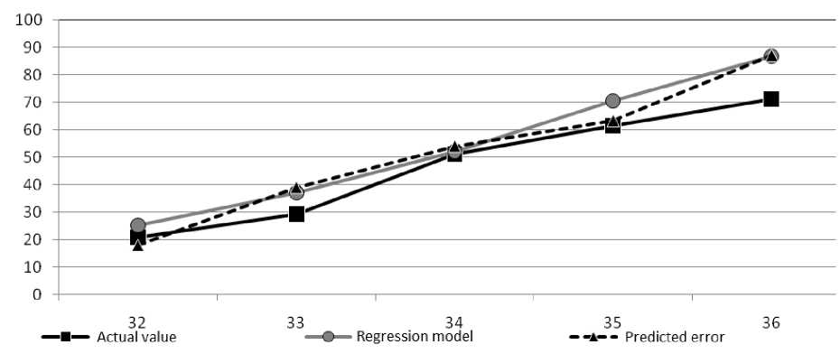
Fig. 4. Graph display of predicted results

• Рис. 4. Графическое отображение результатов прогноза

The values of the average approximation error for Y_t ,

• Y_t ^′ and Y_t + e_t ′ are the following:

• 1)    A ( Y t ) » 17,03%;

• 2)    A ( Y_t ′ ) ≈ 71,18 %;

• 3)    A ( Y t + e t ) » 15,59%.

The highest indicator of the average approximation error was obtained under the assumption that the time series Y t is a random variable. The average approximation error for the regression model is 54.15 % less, which tells us that the time series is a determinate value. As a result of including values e_t ′ in regression, the average approximation error decreased by approximately 1.44 %.

Conclusion . The method presented above can be used to determine the continuous distribution function of a random variable and generate a random variable for predicting and simulation purposes.