Thresholding or Bayesian LMMSE/MAP estimator, which one works better for despeckling of true SAR images?

Published Online January 2019 in MECS DOI: 10.5815/ijigsp.2019.01.01

In synthetic aperture radar (SAR) imaging system high resolution images of stationary targets on the ground are produced by transmitting electromagnetic waves and coherent integration of received echoes. Since multiple backscattered echo pulses are coherently processed in this system, the random interference of electromagnetic waves causes the speckle noise [1]. Speckle is well modeled as a multiplicative noise which degrades the quality of SAR images, and therefore, despeckling is one of the important tasks in SAR imaging systems. The purpose of image despeckling is to remove noise while retaining the important image features. Classical despeckling algorithms such as Lee [2] and Frost [3] methods are based on priori statistical information of speckle noise and usually over-smooth the textures. In recent years, with the development of multi-resolution analysis theory, transform domain-based techniques such as wavelet and contourlet transforms (CT) are utilized for despeckling purposes [4-5]. The non-subsampled contourlet transform (NSCT) proposed in [6], is a shift-invariant directional multi-resolution image representation built upon nonsubsampled pyramids and directional filter banks.

The two simple, yet efficient, methods for SAR despeckling are using (i) thresholding (or shrinkage) estimators [7], and (ii) Bayesian estimators such as linear minimum mean square error (LMMSE) estimator or maximum a posteriori (MAP) estimator [8]. The SAR image is first converted into the transform domain like the NSCT. In the thresholding method, a thresholding function is utilized to modify the transform coefficients. The common modification is based on rejecting those transform coefficients that are smaller than a given threshold and keeping the remaining coefficients. Clearly, a thresholding-based despeckling technique would be effective if signal coefficients in transform domain follow a near-sparse representation so that the signal energy can be approximately determined by using a small subset of the coefficients. Two well-known thresholding functions for noise reduction are hard and soft thresholding mappings [6][9]. On the other hand, in Bayesian estimation the aim is to estimate the noise-free transform coefficients from the observed ones and from the statistical knowledge of the signal and speckle distributions. At the last stage of both methods the despeckled SAR image is recovered using the inverse transform.

Despite the fact that thresholding estimators can provide a better visual quality of image reconstruction in comparison with procedures that only use MMSE criteria [9], classical thresholding functions for image denoising suffer from specific drawbacks. A hard thresholding mapping is discontinuous (i.e., not differentiable) and when the noise power is significant it yields abrupt artifacts in the recovered images. Although the soft thresholding mapping is continuous and weakly differentiable (the first derivative exists), such mapping still creates a constant deviation shift between the true and estimated coefficients, which may reduce the quality of the image and result in a blurred image. In addition to the shape of mapping function, finding the optimum value of the threshold is also of great importance. For multiresolution transform based analysis like NSCT, the threshold selection can be adaptive or non-adaptive per subband [7][10].

• A.    The Paper’s Contributions

The main contribution of this paper is two-fold. We first propose a subband-adaptive thresholding estimator for SAR image despeckling in NSCT domain utilizing a new mapping function with two optimally determined threshold values. The new mapping function provides a mathematically continuous input-output relationship to overcome the drawback of hard thresholding mapping, and when input coefficients are larger than the second threshold, leads to a smaller deviation between the input and estimated output coefficients to overcome the drawback of the classic soft thresholding mapping. The performance of a typical denoising algorithm is commonly evaluated in terms of both the speckle removal ability and the edge saving efficiency. Experimental results illustrate that the new thresholding estimator improves the denoising performance in comparison with other existing thresholding methods. However, still a Bayesian LMMSE/MAP estimator can provide greater speckle removal efficiency in noisy images with high power speckle, and some thresholding methods produce higher edge saving efficiency. This motivates joint exploitation of the superior edge saving ability of thresholding estimators and the greater speckle removal efficiency of the Bayesian estimators, to develop a combined despeckling algorithm in the second part of the paper. To this aim, we utilize the edge information of the noisy image (extracted using a typical edge detection algorithm) to select the output of the combined despeckling algorithm at a multiplexing decision mode with two despeckled images as the input. In particular, when the position of a pixel is recognized as an edge location the corresponding output pixel of the thresholding estimator is selected and in other cases the output pixel of the Bayesian estimator is chosen as the final element of the despeckled image. Simulation results over real SAR images show that using a combined approach is more effective in test image scenarios with high power speckle.

• B.    Related Works

It is worthy to note that in the literature there exist several transform-based state-of-the-art denoising methods that are more sophisticated and complex compared to thresholding estimators (see, e.g., [11-12]). Although these methods provide better denoising performance, their computational complexity is significantly much higher and in case the speed and time are of great importance we may still prefer to use simple thresholding or Bayesian LMMSE/MAP estimators. As validated in [7], the actual Bayesian estimator for generalized Gaussian distributed data behaves similar to a piecewise linear thresholding (shrinkage) function. Therefore, it is of special interest to provide simple optimized shrinkage functions for SAR denoising purposes. In this direction, several studies focused on the design of shrinkage functions to overcome the limitations of hard and soft thresholding mappings [7][13-15]. For example, in [7] a parametric piecewise linear shrinkage function denoted by rigorous BayesShrink (R-BayesShrink), is proposed and the optimum values of the shrinkage parameters are calculate by minimizing the least square error between the actual Bayes estimator and the piecewise linear shrinkage function. As illustrated in [16] and [17], when the transform coefficients of noise-free signal and speckle are modeled using generalized Gaussian distributions, closed form solutions for the MAP estimator can be obtained with a limited computational cost. Moreover, the LMMSE estimator is a first-order approximation filter that involves moments up to the second order of the noise-free signal and speckle NSCT coefficients and does not depend on the statistical distributions of the transform coefficients [8].

The rest of this paper is organized as follows. Section II presents the preliminaries including basic modeling and utilized tools. The new proposed thresholding function is introduced in Section III. Section IV presents the idea of combined despeckling algorithm using the edge information of the SAR image. Section V provides performance evaluation over real SAR images, and finally, the concluding remarks are presented in Section VI.

• II.    Preliminaries

In this section brief descriptions are presented for basic concepts and tools utilized in the paper. In particular, a statistical model for the speckle noise is described and, the NSCT and thresholding methods in the transform domain are introduced briefly.

• A.    Speckle Noise and Image Statistics

Assuming that a natural fairly regular surface seen by the radar, each SAR image pixel from this surface includes the effect of a large number of elementary scatterers, where backscattered echoes add to each other coherently. The total pixel response in amplitude and in phase is the result of these backscattered echoes contributions in the complex plane [1]. More precisely, when an electromagnetic wave scatters from position (x, y) on the target surface, both the phase, φ(x,y), and amplitude, A(x,y), of the wave experience some changes depending on the characteristics of the terrain. In this case, the local reflectivity at each pixel can be represented the number pair (Acos(φ), Asin(φ)) measured on the in-phase and quadrature channels of the SAR antenna receiver. When the local reflectivity at each pixel is represented by the complex number Aejφ = Acos(φ)+jAsin(φ), the SAR data is known as the complex image. In practice, it is easier to interpret the images of the amplitude A and the intensity u = A2. As described in [1], speckle is known as the noise like quality characteristic of the aforementioned types of SAR images. From the statistical perspective, the complex reflectivity Aejφ at each pixel may be modeled as the sum of a large number of complex backscattered echoes as follows:

Ae j = X + jY = ]T A_ke" k             (1)

k = 1

where Ak and ^ are the amplitude and phase of the kth scatterer and N is the total number of scatters in pixel. To provide a simple speckle model the following assumptions are made: (i) the response of different scatterers are independent; (ii) for each scatterer the amplitude A and the phase %. are independent; (3) the variables Ak have the same probability density function (PDF); and (4) the phases %. are uniformly distributed between —n and n. According to the central limit theorem, the real and imaginary parts of the complex reflectivity in (1), i.e. X and Y, are independent zero mean random Gaussian variables with variance ст /2 for large N. Hence, the speckle amplitude A has the Rayleigh distribution and the PDF of the  intensity I = A2 = X2 + Y2 follows  an exponential distribution  p(I) = 1/ ст exp(—I / ст), I > 0

with the average E ( I ) = ст and the variance Var ( I ) = ст ² . In L -look SAR image processing, L independent observations of the same area are averaged and therefore the intensity I is modeled by a Gamma Г ( L , L )

distribution as follows [1] (such averaging preserves the mean value of the total intensity while reducing its variance by a factor L ):

L

P ( I ) =      I - I I L exp( - LI / ст )-    I >  0   (2)

^{Г ( L} ) l ст )

with mean value E ( I ) = ст and variance Var ( I ) = ст ² / L .

In this article, we consider the following model for SAR images corrupted by multiplicative speckle (see Eq. (4.15) from [1]):

g ( n ) = f ( n ). I ‘ ( n ) = f ( n ) + f ( n ) [ I ‘ ( n ) — 1 ] = f ( n ) + N ( n )

where g ( n ) and f ( n ) are the observed noisy signal and the noise-free surface reflectance at pixel position n= [ n 1 , n 2 ], respectively, and I′ ( n ) is the fading variable (speckle) which is a stationary random process independent of f , with unit mean value. The term N ( n ) = f ( n ). [ I '( n ) — 1 ] represents an additive zero-mean signal-dependent noise term, which is proportional to the signal to be estimated. Since f ( n ) in nonstationary in general, the additive noise N ( n ) will be nonstationary as well.

• B.    NSCT and Thresholding Estimators

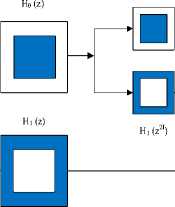
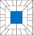
The NSCT is a multiscale multiresolution transform which can be basically divided into two shift invariant parts: (i) a nonsubsampled Laplacian pyramid structure that ensures the multiscale property, and (ii) a nonsubsampled directional filter bank (DFB) structure for directional decomposition. Using such a structure, NSCT splits the two-dimensional frequency plane into several subbands [6]. Fig.1 (a) depicts the decomposition framework of NSCT using a filter bank structure that splits the frequency plane into subbands in two levels (scales) according to the frequency partitioning illustrated in Fig.1 (b). The input is first split into a low-pass subband and a high-pass subband using a nonsubsampled pyramid structure. The high-pass subband is then decomposed into several directional subbands using the DFB structure. By repeating the operation on the low-pass subband one may obtain an arbitrary number of decomposition levels. It should be noted that NSCT is a redundant and shift invariant image decomposition with efficient implementation that can provide a better frequency selectivity and regularity compared to the contourlet transform [5]. As is verified in [6], the NSCT leads to a better deniosing performance compared to competing transforms such as the nonsubsampled wavelet transform and curvelet transform. In fact, contourlet transform could represent edges and other singularities along contours more efficiently and therefore using NSCT the speckle noise can be separated from the original image more easily.

image

H 0 (z^2I)

( a )

Low pass subband

Band pass subband

High pass subband

( b )

Fig.1. (a) The filter bank structure that implements the NSCT using the high-pass filter H 1 ( z ) and the low-pass filter H 0 ( z ) in two levels; (b) A 2D frequency partitioning with a low pass subband, four, and sixteen directional subbands at levels 1 and 2, respectively.

Since the NSCT is linear transformation, transform coefficients of noisy image in Eq. (3) are divided into two parts:

W_g ^{j - k ]} ( n ) = w [^j - ^{k ]} ( n ) + W_N j - ^{k ]} ( n )           (4)

where W[j,k](n), W[j,k](n), and W[j,k](n) denote NSCT coefficients of g(n), f(n) and N(n) at level number j and directional subband number k, respectively. The basic idea behind the thresholding-based deniosing method in transform domain is that when the coefficients of the original image, i.e., W[j,k](n), are large and concentrated, and in contrast the noise coefficients, i.e., W[j,k](n), are small and dispersive, then using an accurate threshold one can obtain a reasonable estimate of noise-free coefficients W[ j,k] (n). Here, we explain this simple idea using well-known hard- and soft-thresholding estimators. To simplify the notation, in the following we use the short notation 6 = W[j’k] (n), x = W[j,k] (n), v = W[’,k] (n) for estimation purposes in the NSCT domain. The hard-threshold function (also called the shrinkage function) provides an estimate of the noise-free NSCT coefficient θ using the following mapping:

0 ( x ) =

0, x ,

| x | < X | x | > X

In NSCT domain, the threshold in (7) is calculated individually for each pair ( j , k ) where the indices j and k indicate the level and the directional subband numbers, respectively. The main difference between wavelet and contourlet domains is that the former is an orthogonal transform, and therefore it would be enough to estimate the noise variance at the highest frequency subband [7]. However, since NSCT is not an orthogonal transform, in this case we need to estimate the variance of noise in different levels and directional subbands individually. To make the threshold (7) data-driven, the parameters ct₆ and CT, ² are estimated from the observed data as follows. The noise variance ct V is estimated using the median absolute deviation (MAD) estimator as:

where λ is a threshold.

On the other hand, the soft-

threshold function for the estimation of θ is:

„ ₂   [ Median ( x ) )

CTV = v (  0.6745  )

0 ( x ) = 1

f o,

X

⁽¹ —) ^x, x

| x | < X

| x | > X

Since the speckle and the image signals are independent and the NSCT is a linear transformation, the variance of the noisy data can be expressed as [19]:

2  2,2

CTx = CT6 + CTv

• III.    A New Thresholding Estimator

Classical shrinkage functions such as hard- and soft-thresholding suffer from specific drawbacks in image denoising applications. To overcome these drawbacks in this section, we propose a new mapping function with two optimized thresholds. As mentioned before, in the design of thresholding estimators finding the optimum value of the threshold is an important task. For example, the threshold in the SureShrink method derived by minimizing Stein’s unbiased risk estimate in a subband-adaptive manner [18]. One other distinguished threshold is the BayesShrink, derived from minimizing a Bayesian risk at each decomposition level and for every subband separately [10]. Here we first describe the BayesShrink threshold in brief, originally developed in the wavelet domain.

• A. BayesShrink Threshold Selection

As verified in [10], given that the signal and noise wavelet transform coefficients are distributed according to generalized Gaussian and Gaussian PDFs, respectively, using numerical calculation a nearly optimal threshold (called BayesShrink threshold) can be found as:

ст ²

X = -^                  (7)

^CT 6

where ct₆ is the standard deviation of the noise-free image transform coefficients and ст ,2 is the variance of noise transform coefficients. It is demonstrated that the threshold in (7) yields a risk within 5% of the minimal risk over a wide range of parameters of assumed prior distributions [10].

Moreover, the variance of the noisy data CT2 can be estimated as follows:

CT ² =   ¹— X( x ( n ) - m, ) ²          (10)

x M x N^n        x’ where M x N is the image size, and mx =^ x (n)/(M x N) is the estimation of the mean n value E[x]. From (9) and using (8) and (10), the standard deviation of the noise-free NSCT coefficients can be estimated as:

<Т б = ^max ( с т x ^- с т,,⁰ )

x

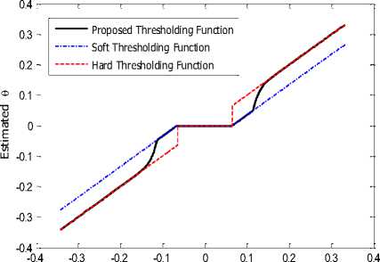
Fig.2. The graph of the thresholding function in Eq. (12). The horizontal axis depicts the range of NSCT coefficients in a sample NSCT subband. The thresholding functions in Eqs. (5) and (6) are also depicted.

B. New Threshold Function

The new mapping function is mathematically continuous and creates asymptotically a zero deviation between the input and estimated output coefficients when input coefficients are large. The proposed mapping function is given by:

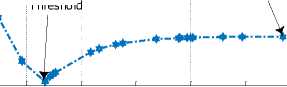
X₂ which satisfies the condition |ct 2 (X₂) - o 2| <  £ for a predefined small tolerance ε (see Fig.3 (b)). Since the parameter estimation is data-driven, in practice we have to solve the problem (13) numerically. To this aim, the following bisection-like algorithm is developed to find the optimum threshold λ in a target NSCT subband.

9 ( x ) = 2

0, sign(x)(| x I -A), 1x3

. sign ( x )(| x | A ^A ),

| x < ^ A <| x |< A

A ₂ < | x |

Fig.2 depicts a typical graph of the function (12). In each subband two threshold values λ and λ are utilized.

In the interval | x | <  A all input coefficients shrink to zero in accordance with common hard- and soft-thresholding estimators. In the interval X <  | x | <  X₂, a mapping similar to that of soft-thresholding method is utilized (see Eq. (6)). For the interval | x | >  X₂ , a nonlinear mapping which asymptotically converges to sign ( x ). | x | for large x , is employed (note that in all practical situations the condition X₂ <  1 should be held) which is in agreement with zerodeviation property of hard-thresholding mapping (see Eq. (5)). The first threshold λ is selected as the BayesShrink threshold in Eq. (7). The second threshold could be in the ^interV^al   X , e^ , ^X max ]   , ^{where X}_mn = I j    ^and

X   =| x  | (< 1) is the maximum value of NSCT max     max cofficients in the considered subband. Clearly, for X2 = X^, the mapping function in (12) acts as the soft-thresholding function. Moreover, for X2 = Xmin the mapping function in (12) leads to estimation results which is very close to that of the hard-thresholding function. To attain the best despeckling performance, the optimum λ is calculated by solving the following optimization problem:

X₂ = arg min л ² (X 2 ) - o^             (13)

λ 2

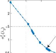
where ст_в ² is the variance of the noise-free NSCT coefficients estimated by (11), and ст -² is the variance of the NSCT coefficients after despeckling. The variance ст -² can be estimated using an equation similar to (10) from NSCT coefficients θ^ˆ . Figs.3 (a) and (b) depict the estimation of ст -² and the difference |o ? (X₂) - o2| with respect to the treshold λ for a sample subband, respectively. Our observations verify that the curve of ст -² versus λ is always decreasing when the threshold λ increases. Moreover, there is an optimum threshold value

Algorithm 1:

InPut : ^X min , ^X max , ^CT e , ^tolerance £

Output : λ_opt

1-

2-

3-

4-

5-

^{Set X} 2,1 = ^X min , ^X 2,2 = ^X max

.

Calculate the new threshold value λ

_ X2,1 + ^X 2,2 ‘ 2,new

.

Use Eq. (12) to despeckle the target subband and calculate ²          .

θˆ 2, new .

If  l^ 2,new ) — n 2|

ε STOP. The solution is

opt       2,new .

If  °e (X2,new) > °e replace X2,1 = X2,new   and if ne (X2,new) < ne replace X2,2 = X2,new.

Repeat step 2 to step 5.

IV. A Combined Thresholding/Bayesian Despeckling Algorithm

In a thresholding method like hard thresholding, it is assumed that the small coefficients bellow a given threshold are dominated by noise, and therefore such coefficients are set to zero. Since edge locations at an image are related to large transform coefficient amplitudes, the output despeckled image of a hard thresholding method still contains a large percent of the original edge information as at the noisy image. However, since coefficients above the given threshold remains as they were, residual noise still presents in the resulted despeckled image. On the other hand, although Bayesian LMMSE/MAP estimators have great speckle removal efficiency they provides a relatively poor edge preserving performance especially at high levels of the speckle power [20] (our results in rows 1 and 2 in Table 2

x 10-3

2.5

Estimated Optimal Threshold

0.5

Soft

Thresholding

-♦-♦#•■

0.05

0.1

0.15

^2

(a)

0.2

0.25

0.3

0.35

1.8

1.6

x 10

1.4

p ^{( 9 )} = "l^exp V 2 ct₉

_ V2 9 - ц6\

.         ст0

,

1.2

0.8

0.6

0.4

0.2

P ( V ) =

V V

X

0.05

—;=— exp I---

2ПСТсту    (  2ст

Estimated Optimal Threshold

Soft

Thresholding

0.1

0.15

0.2

0.25

0.3

^ 2

(b)

where ^ = E [ 9 ] = E [ x ]. Using (15), the MAP estimator for the noise-free component θ is given by [17]:

0.35

Fig.3. (a) Variance of the NSCT despeckled coefficients ² , and (b) the 9

difference between the variance of NSCT despeckled coefficients and the estimated variance of noise-free NSCT coefficients, | ° 2 ^(X2 ) - ^ce , versus X 2 for a sample subband.

also confirm this claim). In this section, we aim at joint exploiting of the good edge preserving performance of thresholding methods and great speckle removal efficiency of Bayesian estimators, to design a more powerful despeckling algorithm.

A. Low-Complexity Bayesian LMMSE/MAP Estimators

Since the noise-free image signal and speckle are uncorrelated from Eq. (1) the LMMSE estimation of the noise-free image denoted by <9 = W [ j ^, k ^] ( n ) can be expressed by [8]:

B. Despeckling Algorithm

9 = E[9]+

= E [ x ] +

cov( 9 , x ) var( x )

.     ^ct 9

^9 + ^v

( x - E [ x ] )

( x - E [ x ] )

where x = W j ^{, k ]} ( n ) and v = W ^[ j ^{, k ]} ( n ) . In [19] it is demonstrated that for the noise component we have E [ v ] = 0, and therefore from (4) we obtain E[ 9 ] = E [ x ]. As evident from (14), the LMMSE estimation only depends on the first and second order moments of the image and noise signals. In subsection 3.1 the procedures to estimate the statistical moments E [ x ], ст 2 , and ct V , have been discussed.

As in [17], to limit the computational cost and also to attain a closed-form solution for the Bayesian MAP estimation, we utilize the Laplacian and Gaussian distributions for the NSCT coefficients of the noise-free image and noise signals, respectively, as follows:

>     . V2 ст -²

x ^ Цв +   - ств

-CTctV

—

ue elsewhere

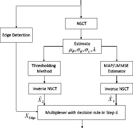
In the proposed despeckling algorithm depicted in Fig.4, the LMMSE/MAP and thresholding estimators are first separately utilized to produce two despeckled images denoted by x ˆ and x ˆ , respectively. Then, based on the

edge information of the pixel positions, these two images are combined and the despeckled output image is constructed. For the edge detection, we use of the Canny method [21]. The algorithm consists of the following basic

steps:

Algorithm 2:

Input : Noisy Image ( X )

Output : Denoised Image ( Y )

1. Extract the edge information at the noisy input image (it is denoted by X ).

Apply NSCT to decompose the input noisy image into sub-bands.

Estimate the statistical required parameters and calculate the optimum threshold.

Implement the LMMSE/MAP Bayesian and thresholding estimators separately over the NSCT coefficients.

Apply inverse NSCT to obtain the output pixeldomain images from the LMMSE/MAP estimator ( X ˆ ) and the hard thresholding estimator ( X ˆ ).

At pixel position n= [ n 1 , n 2 ], decide based on the edge information X ( n ) as follows:

• •    If position n is an edge pixel, set Y ( n ) = XX ₂( n ) .

• •    If position n is a pixel in smooth region, set

Y ( n ) = J X j ( n ).

Noisy Image: X

Noiseless Image: Y

Fig.4. Flowchart of the proposed combined despeckling algorithm. Here, the edge information of the pixel positions in the original noisy image is utilized to select the final pixel element of the despeckled image from the outputs of thresholding and Bayesian estimators.

• V.    Experimental Results

In this section, experimental results are provided and compared with other depeckling methods with approximately the same computational burden. The performance assessment results are presented for real SAR images with natural speckle noise. In NSCT implementation we use four scales and 4, 4, 8, 8 directions in the scales from coarser to finer, respectively. Moreover, in applying a thresholding method in the NSCT domain the denoising operation is performed over coefficients of high-frequency subbands. For the LMMSE and MAP estimators, we use a local window with dimension 11 × 11 to calculate the local variance of the noisy data as in [22].

• A.    Quality Assessment Criteria for Despeckled Images

In the literature, several metrics for image quality evaluation are proposed that can be utilized to quantitatively assess filtered images. These metrics cover various aspects of denoising algorithms such as noise reduction, edges and feature preservation [23]. The equivalent number of looks (ENL) is defined as follows:

ENL =

( ^mean( f H ) ) var( f ^ˆ _H )

where fˆ refers to the despeckled image at the selected homogeneous region. The ENL of the filtered SAR image is compared with respect to the ENL of the original noisy image. The ENL is a measure of speckle removal ability of the applied algorithm such that a higher ENL indicates a better despeckling efficiency.

In addition to speckle removal capability, another metric which is utilized to represent the edge preservation capability of the despeckling technique is the edge save index (ESI) [24]. ESI indicates the ratio between the gradient of the filtered image and the original (noisy) image edges and its range is [0,1]. This metric can be computed in both horizontal ( ESI^h ) and vertical ( ESI^v ) directions of the despecking algorithm as follows:

M N - 1

SS| f i , j + 1] - f i , j ]

ESIh = та-------------

SSI L [ i , j + 1] - f o [ i , j ]| i = 1 j = 1

M-1 N ..

SS| f [ i + 1, j ] - f [ i , j ]|

ESIv=M^-N (19)

SSI fo [ i + 1, j ] - fo [ i , j ]| i = 1 j = 1

where f ˆ is the denoised image and f refers to the original (noisy) image. A larger ESI indicates that the original image’s edges have been preserved better after speckle removal.

• B.    Results for true SAR images

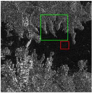
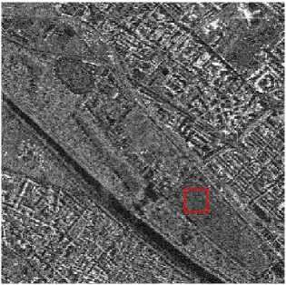
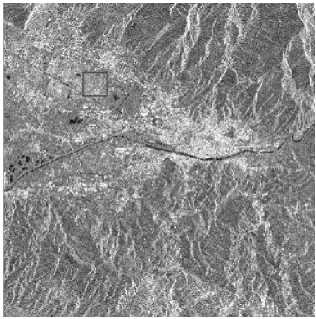
For experiments, we consider three SAR images in amplitude format taken with different number of looks: (i) KOMPSAT-5 one-look image of Sydney [25], (ii) original COSMO-SkyMed 4-look StripMap image [23], and (iii) original 5-look ERS-2 image [23] (see Fig.5). Since the speckle power in a SAR image is conversely proportional with the number of looks, naturally a one-look image is contaminated with a more powerful speckle. For all images, the ENL and ESI parameters are computed as follows. To calculate the ENL, for each test image a homogeneous region in the image is selected, indicated in the red box in Fig.5. The ESI parameters are calculated over the whole image. The despeckling results for thresholding algorithms are reported in Table 1. For the performance evaluation purposes, the results are also reported for several existing thresholding estimators previously presented in the literature. Since the performance of the Hashmi’s thresholding function [7] depends on the internal parameter β , we depict its results for three different β .

As evident from Table 1, there is a basic tradeoff between the performance metrics ENL and ESIs for different thresholding functions. This means that an estimator that increases the ENL in comparison with the reference estimators such as soft-thresholding (ST) and hard-thresholding (HT), it essentially decreases the ESI parameter. For instance, both Zhang [13] and Nasri [14] estimators provide better ESI parameters w.r.t the HT estimator, however the latter produces a higher ENL metric. In comparison with other existing thresholding estimators, in general our estimator provides a better tradeoff between the performance metrics ENL and ESI. For example: (i) The ENL of the proposed thresholding function and ST are approximately the same for different test images, however the former estimator leads to higher values of ESIs; (ii) Both the ENL and ESIs metrics of the proposed estimator are better than that of the Hashemi’s estimator with β=1.5; (iii) The proposed estimator acts better when compared with Chuia’s estimator for both 4 and 5-look SAR images, however in case of 1-look image, it only provides a better ENL parameter.

In Table 2 we report the despeckling results of the proposed combined algorithm in Fig.4 in addition to the results of pure LMMSE and MAP estimators. The combined schemes are specified by the two part names. For example, the name HT–LMMSE refers to the combination of the HT and the LMMSE estimators, and the name Pro–LMMSE (MAP) refers to the combination of the proposed thresholding method and the LMMSE

(MAP) estimator in Fig.4. By comparing the results of pure LMMSE and MAP estimators in Table 2 with those reported in Table 1, one can observe that when the speckle power is higher in the test image (i.e., the one-look image), the pure LMMSE and MAP estimators produce larger ENL values w.r.t. all thresholding estimators. Of course, for the test images with lower speckle power (e.g., the 5-look image), still the proposed thresholding estimator provides a higher ENL value w.r.t. the Bayesian estimators. We should also note that the best edge efficiency (higher ESI values) is always produced by the HT estimator in Table 1.

Moreover, from the results in Table 2 it is evident that: (i) the combined HT–LMMSE scheme produces the best ESI results in all cases of the test image. This is quite expected because the HT estimator has the best edge preserving efficiency (higher ESI values) among all other thresholding estimators (see Table 1); (ii) when the speckle power is high

(a)

(b)

(c)

Fig.5. (a) KOMPSAT-5 one-look image taken over Sydney. (b) Original COSMO-SkyMed 4-look StripMap image. (c) Original 5-look ERS-2 image of Florence.

Table 1. Speckle noise reduction results for three different real SAR images using different thresholding estimators.

Image Under Test	one-look KOMPSAT-5			4-look COSMO-SkyMed			5-look ERS-2
	ENL	ESIh	ESIv	ENL	ESIh	ESIv	ENL	ESIh	ESIv
Original Image	2.6	1	1	15.06	1	1	25.37	1	1
Hard Thresholding (HT)	31.59	0.864	0.862	86.94	0.502	0.607	50.30	0.458	0.471
Soft Thresholding (ST)	45.91	0.495	0.491	90.54	0.311	0.342	63.52	0.267	0.245
Zhang-HT [13]	31.72	0.855	0.851	86.98	0.502	0.607	50.71	0.458	0.471
Zhang-ST [13]	42.00	0.506	0.504	90.06	0.316	0.348	62.74	0.273	0.253
Nasri [14]	38.34	0.764	0.761	89.09	0.424	0.506	55.25	0.379	0.381
Chuia [15]	44.45	0.671	0.665	90.40	0.356	0.406	60.11	0.310	0.298
Hashemi [7]: β =0.5	46.86	0.377	0.374	90.91	0.292	0.306	65.40	0.250	0.223
Hashemi [7]: β =1.5	43.40	0.561	0.559	90.50	0.320	0.361	62.51	0.275	0.256
Hashemi [7]: β =2	40	0.601	0.601	90.36	0.324	0.372	61.64	0.278	0.261
Proposed Thresholding:	45.90	0.587	0.579	90.53	0.389	0.430	63.47	0.336	0.321

Table 2. Speckle noise reduction results for three different real SAR images using different combined estimators.

Image Under Test	one-look KOMPSAT-5			4-look COSMO-SkyMed			5-look ERS-2
	ENL	ESIh	ESIv	ENL	ESIh	ESIv	ENL	ESIh	ESIv
Original Image	2.6	1	1	15.06	1	1	25.37	1	1
LMMSE	47.57	0.577	0.573	89.87	0.445	0.473	56.12	0.411	0.400
MAP	46.95	0.478	0.476	90.35	0.377	0.402	59.45	0.336	0.318
Hashemi–LMMSE ( β =1.5)	47.57	0.573	0.569	90.23	0.428	0.457	58.02	0.391	0.376
Hashemi–MAP ( β =1.5)	46.91	0.502	0.500	90.46	0.368	0.395	60.37	0.326	0.307
Chuia–LMMSE	47.57	0.625	0.602	90.26	0.431	0.465	57.79	0.395	0.382
Chuia–MAP	46.93	0.538	0.536	90.48	0.374	0.405	60.13	0.331	0.314
Nasri–LMMSE	47.51	0.633	0.630	90.39	0.443	0.481	57.04	0.406	0.397
Nasri–MAP	46.93	0.568	0.567	90.62	0.394	0.425	59.31	0.345	0.331
ST–LMMSE	47.54	0.556	0.551	90.20	0.427	0.454	58.11	0.391	0.375
ST–MAP	46.91	0.484	0.481	90.43	0.367	0.392	60.47	0.326	0.305
Zhang-HT–LMMSE	47.49	0.558	0.554	90.17	0.428	0.454	58.03	0.391	0.376
Zhang-ST–MAP	46.90	0.486	0.484	90.40	0.368	0.393	60.38	0.326	0.307
HT–LMMSE	47.58	0.665	0.662	90.56	0.461	0.503	58.02	0.442	0.456
HT–MAP	46.97	0.601	0.600	90.79	0.415	0.451	59.74	0.366	0.354
Pro–LMMSE	47.57	0.576	0.572	90.19	0.436	0.463	57.83	0.381	0.373
Pro–MAP	46.91	0.505	0.503	90.42	0.378	0.404	59.61	0.336	0.320

(i.e., the one-look image), the combined HT–LMMSE scheme also provides the best ENL result w.r.t. other combined schemes. This is also quite expected because in high speckle power the pure LMMSE estimator creates the best ENL result. As a result, in high speckle power scenarios the best ENL and ESIs results are provided by the H–LMMSE scheme; (iii) When the speckle power is low (e.g., 4 and 5-look images), the best ENL result is provided by the ST–MAP scheme (60.47) which is smaller than that of the proposed thresholding estimator in Table 1 (63.47). Hence, in such cases our proposed thresholding estimator is the best despeckling algorithm among all discussed schemes; (iv) As the final note, we observe that the HT-MAP and HT-LMMSE schemes produce better ENL and ESI performance w.r.t the pure LMMSE/MAP estimators, which in fact confirms the efficiency of the combining idea in Fig.4.

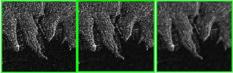
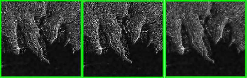
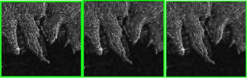
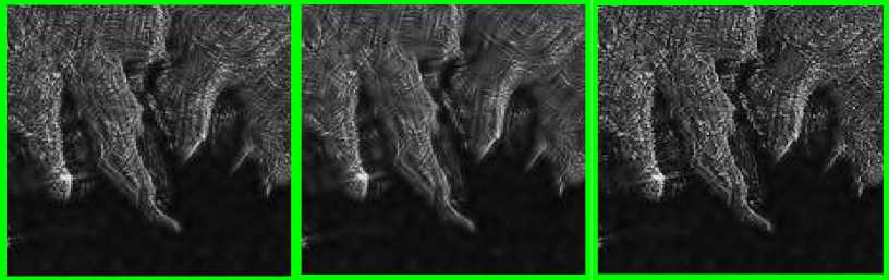
In Fig.6, a visual comparison between the output images of the proposed and benchmarking estimators is presented for a rectangular selected green area from the KOMPSAT-5 one-look image (see Fig.5 (a)). From this figure, one can see that the proposed HT-LMMSE scheme provides better despeckling results than other despeckling methods in terms of visual quality, i.e., it produces a smoother image and preserves the edge information more efficiently. Moreover, it does not make additional artifacts in the despeckled image.

(a)                                          (b)                                          (c)

(d)                                              (e)                                              (f)

(g)                                              (h)                                              (i)

(j)                                                  (k)                                                  (l)

Fig.6. Despeckling results for KOMPSAT-5 one-look image: (a) selected green rectangular area from original noisy image (see Fig.5. (a)), (b) hard thresholding, (c) soft thresholding, (d) Nasri, (e) Zhang-HT, (f) Zhang-ST, (g) Chuia, (h) Hashemi (β=1.5), (i) proposed thresholding, (j) LMMSE, (k) MAP, (l) HT-LMMSE.

• VI.    Conclusions

In this paper, we have investigated the SAR despeckling performance of two classes of low-complexity denoising algorithms including the thresholding and Bayesian LMMSE/MAP estimators. Specifically, two efficient denoising algorithms based on pure thresholding and combined thresholding/Bayesian estimation in the NSCT domain are proposed. In the design of the proposed thresholding function, an optimization-based threshold selection approach is utilized at an adaptive manner. In the proposed combined thresholding/Bayesian scheme a multiplexing decision mode is devised which decides based on the edge information of the image pixels, to select the final pixel elements of the despeckled image. The results demonstrate that compared to other recent existing despeckling estimators with approximately the same computational complexity, the proposed thresholding estimator provides a better despeckling performance in terms of speckle removal (higher ENL) and edge saving (larger ESI) efficiencies in test images with low speckle power. On the other hand, for the test images with high speckle    power    the    proposed    combined thresholding/Bayesian scheme produces better despeckling results.