Through the diversity of bandwidth-related metrics, estimation techniques and tools: an overview

Published Online August 2018 in MECS DOI: 10.5815/ijcnis.2018.08.01

Bandwidth has been a critical and precious resource in various kinds of networks. Having a good estimate of bandwidth is, for example, important for network error detection and diagnosis as well as for efficient operation of bandwidth dependent/data-intensive Internet applications. Some popular examples where knowledge of bandwidth can be valuable are validation of service level agreements, detection of congested or underutilized links and capacity planning support, admission control policies at massively-accessed content servers, network tomography for tracking and visualizing Internet topology, dynamic server selection for downloads, optimized congestion control for reliable transport protocols (e.g. for TCP) and optimized network route selection.

Figure 1 shows an overview of major bandwidth estimation techniques and tools. They mainly estimate one of three related metrics: capacity, available bandwidth and throughput. The latter can, in turn, be divided into achievable throughput and bulk transfer capacity (BTC). The estimation of each metric is associated at least with one estimation technique whereas one and the same metric can also be estimated with several and independent estimation techniques in different ways. Representative examples of estimation techniques used by different estimation tools range from Packet Pair (PP) and Variable Packet Size (VPS) estimating the end-to-end and hop-by-hop capacity, respectively, to Probe Rate Model (PRM) and Probe Gap Model (PGM) estimating the end-to-end available bandwidth to TCP connections or emulations used for measuring end-to-end achievable throughput and BTC metrics. Estimation techniques shown in Figure 1 are represented by several various tool implementations. They all show a wide spectrum of different assumptions, characteristics, advantages and limitations:

• •    Active vs. passive estimation tools

• •    Intrusive vs. lightweight estimation tools

• •    Single-ended vs. double-ended estimation tools

• •    Offline vs. online (or real-time) estimation tools

• •    Ability to measure asymmetric, wireless or highspeed links

• •    Different levels of achievable estimation accuracy

• •    Differences in estimation time needed and probing overhead caused

From the point of a user’s view, the wishing list for an ideal estimation technique and tool is long and manifold, and includes requirements such as accurate, consistent and reliable estimates; low overhead, fast and robust estimation procedures; resilience to both cross traffic and its rapid changing conditions; independence of the measurement end-host performance and system capabilities; and finally, applicability to mixed paths consisting of wired, high-speed and/or wireless links.

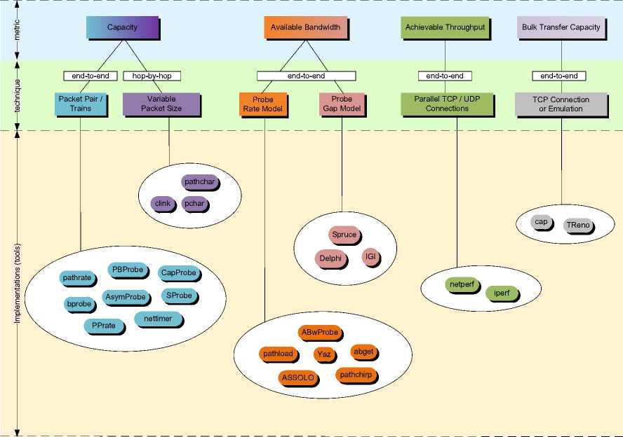
Fig.1. An Overview: Metrics, Techniques and Tools

Current estimation techniques and tools mainly suffer from two categories of challenges that lead to unstable and inaccurate estimates: Challenges that exists in Internet environment such as route alternations, multichannel and asymmetric links, multiple existing bottlenecks, traffic shapers or network components working with non-FIFO queuing disciplines; or challenges which are related to end-hosts performing the measurements such as interrupt coalescence, limited system I/O capability, limited system timer resolution, context switching and clock skew.

The purpose of this paper is (a) to introduce specific bandwidth-related metrics, highlighting the scope and relevance of each; (b) to describe the rationales of the major existing bandwidth estimation techniques; and (c) to survey and uniformly classify the various existing bandwidth estimation tools. Differently from the rest of survey studies in literature [1–3], the focus of this work is

• •    to survey and classify the more recent bandwidth estimation tools

• •    to comprehensively review and critically analyze the relevant characteristics, strengths and weaknesses of bandwidth estimation tools

• •    to give a detailed overview about the challenges, practical issues and difficulties faced by in designing and implementing bandwidth estimation techniques.

The rest of the study is divided into the following sections. Section II describes the four-specific bandwidth-related metrics including capacity, available bandwidth, achievable throughput and BTC. Section III presents the working principles of major bandwidth estimation techniques along with their assumptions. Section IV gives a taxonomy of tools. Section V presents the fundamental challenges, practical issues and difficulties faced by designing and implementing bandwidth estimation techniques Finally, Section VI concludes the paper.

• II.    Bandwidth-Related Metrics

Basically, there exists three popular bandwidth-related metrics: capacity, available bandwidth and throughput. The capacity of a single link is defined as the maximum number of bits this link can transfer per second. If, on the other hand, a path consisting of several links is considered, the end-to-end capacity of this path is given by

Cend - to - end = min Ci (1) i =1... H whereas C is the capacity of link i and H indicates the number of links along the path between the sender and the receiver. In other words, the end-to-end capacity specifies the maximum capacity of the weakest link on the path between two hosts. The capacity is a measure of the bottleneck of a communication link, which is independent of the current load of the network. Figure 2 illustrates a path consisting of three hops whose end-to-end capacity is 64 Kb/s.

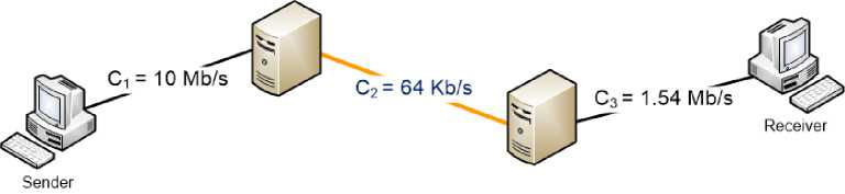
Fig.2. Illustrating End-To-End Capacity of a Path Consisting of Three Hops

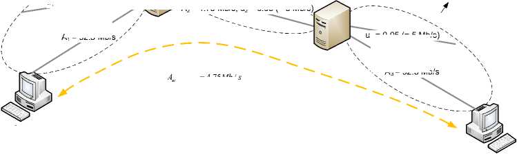
C 2 = 9.75 Mb/s

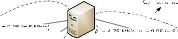
A 2 = 4.75 Mb/s, u 2 = 0.05 (= 5 Mb/s)

C 1 = 97.5 Mbit/s

C3= 97.5 Mb/s u1 = 0.05 (= 5 Mb/s)

A 1 = 92.5 Mb/s

Sender

Receiver

, .   , = 4.75Mb / s end—to—end

Fig.3. Calculating Available Bandwidth Using an Example Scenario at the IP Layer

u 3 = 0.05 (= 5 Mb/s)

A 3 = 92.5 Mb/s

An interesting question when estimating the capacity is on which layer a tool measures this metric. A link on layer 2 normally transports the data at a constant rate. For example, with 10Base-T Ethernet, this constant transmission rate is 10 Mb/s. This is the capacity of this link on layer 2, also referred to as nominal bandwidth. However, as compared to its nominal bandwidth this link provides less capacity to the overlying IP layer because the overhead caused by layer 2 has a reducing effect on the capacity of layer 3. Let C be the capacity of a link on layer 2. The transmission delay of an IP packet of size L byte is calculated as follows:

A

L 3

^LL 3 + ^HL -2

c

L 2

where H represents the layer 2 overhead in bytes. The layer 2 overhead is needed to encapsulate the IP packet to be sent. The effective capacity of this link on the IP layer is:

L^{L 3}        L^{L 3}                 (3)

^{L 3}    a l 3    L l 3 + H l 2

C L 2

It is to be noted that the maximum achievable capacity that is obtained on the IP layer strongly depends on the packet size. Thus, for example, an IP packet with a larger payload size leads to a correspondingly larger capacity, since the overhead of layer 2 has a much greater impact on small payloads than on large payloads. In this respect, it is necessary to use the maximum possible payload size of an IP packet to determine the maximum capacity of the

IP layer. The maximum possible payload size of an IP packet including IP headers is limited by the maximum transmission unit (MTU) for Ethernet. Thus, the capacity on the IP layer is defined as the maximum transmission rate on this layer, which can be achieved using the maximum possible payload size limited by MTU [1].

The available bandwidth of a link can be coarsely defined as the residual capacity on that link during a time interval. The load of the network prevailing at the time of measurement has a considerable influence on available bandwidth. The available bandwidth is determined by traffic from other sources.

Let C be the capacity of link i and Cu the number of bits transmitted via this link during the time interval T . The term U, with 0 <  u <  1 indicates the usage of the bandwidth of the link i during the time interval T . Then, the available bandwidth A of the link i during the time interval T is defined as the fraction of the capacity C which was not used during that time interval.

By extending this concept to the entire path, the end-to-end available bandwidth A           during time end—to — end interval T can be calculated as the minimum available bandwidth among all links, i.e.

^Aend — to — end = min { С Д1 - ^u J}          (4)

i = 1... h

The link with the minimum capacity determines the end-to-end capacity of the path, while the link where the proportion of the unused capacity is minimal limits the end-to-end available bandwidth. The links related to the first and second cases are referred to as narrow link and tight link, respectively.

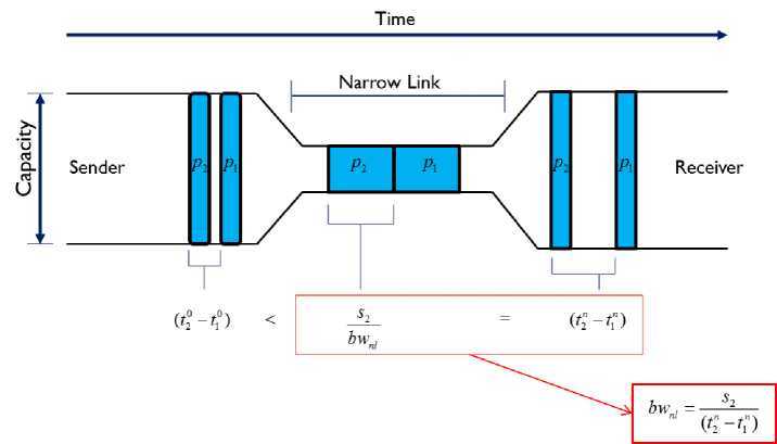
Fig.4. The Rationale of PP Technique [4]

Figure 3 illustrates an example in which the end-to-end available bandwidth is determined considering the layer 2 overhead. It shows a path between a transmitter and a receiver, where the first and third links on the IP layer have an effective capacity of 97.5 Mb/s. The second link has an effective bandwidth of 9.75 Mb/s. The use of this path is constantly 5 Mb/s while measuring the available bandwidth. In this scenario, the end-to-end available bandwidth available at the IP layer is 4.75 Mb/s.

There are two throughput-related metrics, namely achievable throughput and BTC. Both metrics are usually defined for end-to-end paths and measured at the transport layer. Achievable throughput indicates the maximum amount of data that can be successfully transmitted between two hosts over a network. Achievable throughput can be limited by many factors, including hardware properties of the end computers, transport protocol with which the data is transmitted (e.g. TCP or UDP), the non-optimal setting of certain transmission parameters, e.g. for TCP, the size of the buffer at the receiver or selection of the initial size of the overload window, size of the data to be transmitted and RTT of the communication link, to name just a few. The achievable throughput thus indicates the number of bits that an application with these specific settings can maximally achieve. Consequently, it may occur that due to such limitation factors, the achieved throughput of an application is smaller than the actual available bandwidth in the path.

In contrast to achievable throughput, BTC is defined as the maximum rate at which a single TCP connection can send over a given path. The connection should carry out all TCP congestion control algorithms that conform to RFC 2581. TCP throughput depends on various parameters such as congestion control algorithms (i.e. slow-start and congestion avoidance), RTT, nature of side traffic (e.g. UDP and TCP) and flavor of TCP (e.g. Reno, new Reno, SACK). Differently from the achievable throughput which can be measured using different transport protocols such as UDP and TCP and parallel connections, BTC is a TCP-specific metric exhibiting the maximal throughput attainable by a single TCP connection.

• III.    Bandwidth Estimation Techniques

This section presents the details of PP, VPS, PGP, PRM, TCP connection and emulation techniques along with the assumptions each technique makes.

• A.    Packet Pair (PP)

PP estimates the end-to-end capacity between two hosts. Let P be the path between two hosts consisting of n links. The link with the lowest capacity in P is referred to as narrow link, the capacity of which is used synonymously for the end-to-end capacity. PP is based on the fact that if two packets p and p of the same size are queued back-to-back at the narrow link of a path, they leave the link with a time difference of

s

A t =   2—,             (5)

bwnl where the size of the second packet is indicated by s and the capacity of the narrow link is represented by bw . This time difference, also referred to as "dispersion" can be measured at the receiver by subtracting the arrival times of the packet pair (i.e. At = tn - tn )■ By changing the equation (5), the capacity of the narrow link of the path can be deduced, as given in (6). Figure 4 illustrates the rationale of PP technique.

w = то       (6)

t 2     t i

For a correct estimation of the narrow link capacity, PP

Router 1

Sender

Narrow Link

Router 2                   Receiver

s ₂                                        s ₂

bw _nl                             bw _nl

bwnl

s ₂ bw _nl

D)

Narrow Link

< s2- bwnl

> s ²- bw _nl

> s2- bwnl

< s2- bwnl

bwnl

> s2- bwnl

> - s ²- bw _nl

> - s ²- bw _nl

bwnl

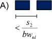
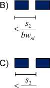
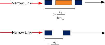
Fig.5. Sources of Error in the PP Estimate [4]

assumes that the two packets are queued back-to-back at the narrow link and that the caused time difference ( t n — t" ) does not change after leaving this link, i.e. there is no queueing after the narrow link. This idealized process is shown in Figure 5-A [4].

However, if the packet pair queued at the narrow link is separated by one or more non-probe packets, the time difference is increased by the size of the additional packets (i.e. the dispersion of the packet pair sample is extended), causing the second packet to fall farther behind than originally caused by the narrow link. In this case, the measured narrow link capacity will reflect a lower value than the actual narrow link capacity. This case is shown in Figure 5-B.

Another error can occur if the first packet p is delayed at the queue of a router after the narrow link by one or more other pre-queued packets, i.e. p must wait longer than p in at least one of the queues of a router after the narrow link, causing the second packet to follow the first packet closer so that the original time difference between the packet pair is reduced (i.e. the dispersion of the packet pair sample is compressed). In this case, the estimated narrow link capacity will reflect a higher value than the actual narrow link capacity. This case is shown in Figure 5-C.

Finally, if the sender initially cannot send the packets close enough together so that they are not queued back-to-back at the narrow link, the time difference between the packets will not clearly indicate the narrow link capacity. In this case, the estimated narrow link capacity will reflect a value lower than the actual narrow link capacity. Figure 5-D illustrates this case.

Cases B through D represent the major sources of error that can occur in a packet pair measurement. Although there are other possible scenarios, these are just combinations of these three cases. Errors of type B to D from Figure 5 cause some noise in the measurement results and should therefore be detected and eliminated.

Several assumptions made by the PP technique must be fulfilled to correctly measure the narrow link capacity of a path. First, the two packets, namely p and p , must have the same size. If p is less than p , then the transmission delay of p would always be smaller than the transmission delay of p . Consequently, the packet p would traverse the individual links in the path to the receiver faster than the packet p , and thus the time difference between the two packets would gradually decrease. If, on the other hand, p were smaller than p , p would traverse the individual links faster than p because of the same reason. In this case, the time difference between the two packets would gradually increase. Second, the packet pair must follow the same path, i.e. no route alternation should occur during the measurement. Third, the routers along the path must process the packets according to the FIFO principle. Finally, PP assumes that the transmission delay is proportional to the packet size and that the routers operate according to the store-and-forward principle.

• B.    Variable Packet Size (VPS)

VPS is used to assess the capacity of each hop within a path between two hosts. This technique starts by sending multiple packets of different sizes to each hop in the path to the receiver and measures the required Round Trip Time’s (RTTs) based on the incoming responses. To measure the RTT, VPS uses the ICMP protocol and performs like the traceroute command, i.e. VPS sends request packets with an increasing TTL value. The start is at TTL = 1. This value is then decremented by each intermediate node on the way between sender and receiver. If TTL = 0, the intermediate node that the packet last reached sends back an ICMP packet of type

11 "Time Exceed" containing the IP address of this intermediate node. In this way, VPS can use the incrementing TTL values to find all intermediate nodes on the way to the destination and can calculate the required RTTs of the packets up to each hop.

According to the VPS technique, the RTT for a packet of size s from node n-1 to node n and back can be calculated as

RTT (s) = qx +1 — + lat I + q2 + forward(7)

f icmp error size .]

+ q₃ + 1-- + lat I + q ₄.

I       bw

The variables q through q represent the random queuing times of a packet and forward indicates the time taken by the forwarding engine to process the arrived packet. To simplify the equation given in (10), VPS makes three assumptions: (i) The size of the ICMP error packet is small enough (56 bytes) that its transmission delay of icmp _ error _ size is negligible; (ii) bw the time taken by the forwarding engine to process an incoming packet is negligible; and finally (iii) if the RTT for a packet size is measured several times, VPS assumes that at least one of these measurements will be performed without queuing delays. In this case, the queuing times q through q can be neglected, too. The elimination of these terms from Eq. (10) yields:

s ) = ^f — + lat | + lat

I bw )                 (8)

= — s + 2 lat.

bw

Eq. (8) represents a linear function with respect to the packet size s , where 1 and 2lat indicate the slope and the y-intercept of this function, respectively.

The VPS method performs the RTT measurement for each hop with different packet sizes. The number of different packet sizes depends on the corresponding VPS implementation. For example, the pathchar [5] implemen-

It is obvious that the measured RTTs for packets with the same size can vary widely. This depends on how long the sent or received packets are delayed in the queues of the individual routers. The shortest RTT for a packet of size s is referred to as Shortest Observed RTT (SORTT). The SORTT for a packet of size s is given by

SORTT ( s ) = — s + 2 lat .          (9)

bw

This linear equation specifies the shortest RTT needed to send a packet of size s to direct neighbor hop. This scenario is shown in Figure 6. However, since the SORTT 's of the different packet sizes on a twodimensional coordinate system are usually not exactly aligned, the required linear function SORTT ( s ) must be approximated. The linear function to be approximated can be determined by using linear regression [6]. Once the optimal linear function SORTT ( s ) = 1— s + 2 lat has been determined, the capacity from the first hop can be determined by computing the inverse of the slope of this approximated linear function, as shown in Eq. (10),

^SloPe SORTT ( s )

A SORTT

:---------------------------------------------------

A s

SORTT - SORTT

^s 2 ^{— s} 1

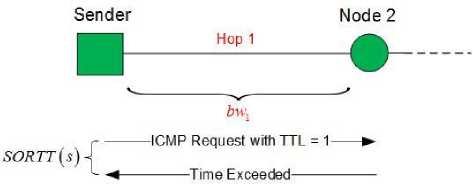
Fig.6. RTT Measurement from Sender to Direct Neighbor Node where (SORTTX, SORTT ) and ( sx, s2 ) are two points on the line approximated by conducting the linear regression.

The capacity of the first hops is thus tation sends a total of n =

MTU

1 different packet

sizes. The MTU for Ethernet is 1500 bytes. Thus, starting with 64 bytes at a distance of 32 bytes, pathchar sends a total of 45 different packet sizes per hop. The RTT measurement per packet size and per hop is additionally repeated p times because of the assumption (iii). Thus, for each hop, pathchar performs a total of p * s RTT measurements.

bw

^slope SORTT(s)

Next, the RTT for a packet of size s is considered from the sender to node 3 via an intermediate node. The scenario is shown in Figure 7.

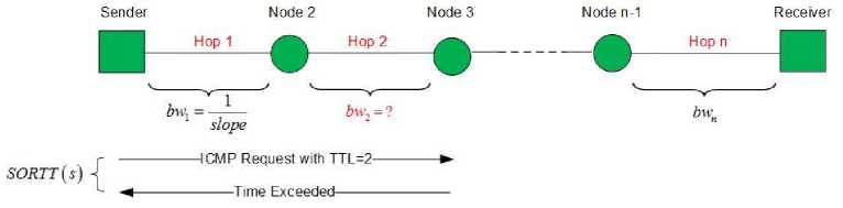
Fig.7. RTT Measurement across an Intermediate Node

The SORTT for a packet of size s from the sender to node 3 is

SORTT ( 5 ) = g     + 2 g lot,

= 5 У--- + 2 У lat, ^g bW j    ^g j

(   1.1    )

= s I ---- +--I + 2 ( lat_Y + lat₂

( bw_x    bw 2 )

As is seen in Eq. (12), the parameters including capacity, slope and latency of the subpath between node 1 through node 3 are formed by the sum of values from each individual hop parameters. Thus, e.g. the term

2 g = 1

1 bw

in (12) represents the slope from the transmitter

n ₁

to node 3. In the following, terms of the type        are

= 1 ^bWj

abbreviated by в . The bandwidth bw_x for the first hop

is given by ¹ The bandwidth bw of the second hop is P 1

then calculated from the inverse of the difference between the two values p and p:

bw2

P2 - Pi

By generalizing the Eq. (13), the capacity bw for the hop j is calculated from:

bw_s =------- ,2 <  j <  n - 1        (14)

j    P j - P j - 1

It should be noted that the slope p given in (14) is also needed to calculate the capacity of the next hop ( j + 1 ) , as for bw applies:

^bw j + 1 = R ¹ R , ² <  ^j <  n - ^{1        (15)}

^P j + 1 - ^P j

For this reason, an incorrect measurement of p. will disturb not only the capacity estimation of hop j but also the one of hop j + 1 .

For VPS, the algorithm must only be implemented on one host, because the RTTs of the sent requests are measured by means of responses at the sender.

As in the case of PP technique, VPS also makes a lot of assumptions to deliver a valid estimate. First, it is required that the ICMP protocol is available on all routers along the path between the sender and the receiver so that all intervening hops can be determined using the TTL Time Exceeded mechanism.

Ideally, each sent packet size should traverse the entire path between the sender and receiver without queuing delay. Failure to meet this requirement for multiple packet sizes can cause the linear relationship between RTTs and different packet sizes to be lost due to random queuing delays.

VPS assumes that the MTU of a link is not exceeded. A packet whose size exceeds the MTU value is fragmented into a certain number of smaller packets. The destination node sends back the ICMP error packet as soon as it receives the first packet of this fragmented ICMP request packet. Since this principle is applied to all other packets whose size is above the MTU, the measured RTTs will be close to each other independent of the packet size. As a result, the determined line that optimally approximates these points will not reflect the correct linear equation for the measurements. In this case, VPS tends to overestimate the corresponding hop capacity.

Measurement conducted by VPS can lead to a significant underestimation of the capacity if the measurement path contains store-and-forward switches. Such devices cause additional transmission delay but do not generate ICMP TTL exceeded messages because they are "invisible" on layer 3. For this reason, this extra transmission delay cannot be considered in the VPS model. The equation given in (15) is only valid for a direct connection between two layer 3 devices. The impact of layer 2 devices on the accuracy of VPS has been further investigated in [7].

Another factor neglected in the model of VPS is the dynamic route change on the Internet. In packet-switched networks, related data packets can reach the destination in different ways. This can happen, for example, if a route is changed dynamically on the way depending on the load situation. In a study conducted by Paxson [8] it has been shown that dynamic route changes on the Internet are very common. Such dynamic route changes during a

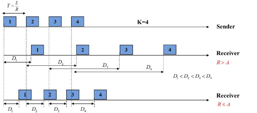
Fig.8. Estimating Available Bandwidth Based on OWD Analysis

measurement can cause VPS to provide false estimates. For example, it is assumed that during the measurement process a route is constantly being changed between two possibilities. Then it may happen that one part of the measurement packets is transmitted via the first possible route and the second part via this second possible route. Since the network interfaces of the two routes can have different capacities and characteristics, the complete measurement of VPS will be falsified.

• C.    Probe Rate Model (PRM)

PRM estimates the end-to-end available bandwidth between two hosts. This technique requires a cooperative environment to perform a measurement, i.e. the sender and the receiver must cooperate with each other, so the measurement software must be used on both sides.

Let P be the path between two hosts consisting of n links. The link with the lowest available bandwidth in P is referred to as tight link, the available bandwidth of which is used synonymously for the end-to-end available bandwidth. The sender begins by sending a sequence of packets to the receiver. This packet sequence consists of K-packets, where K is the length of this sequence. The size of each packet in this sequence is L bits and is periodically sent every t second. The transmission rate of this packet sequence is thus r = L ь / *.            (16)

The sender provides each packet i with a timestamp t before its transmission. Let a be the arrival timestamp of packet i at the receiver. For each incoming packet i , the receiver first calculates its relative one-way delay (OWD) D :

D = ai- t             (17)

For a packet sequence of length K, the receiver calculates a total of K OWDs D , D ,..., D .

12    K

Afterwards, the receiver checks the sequence of these calculated OWDs to deduce whether the transmission rate R of the packet sequence is higher than the available bandwidth A of tight-link. The way in which the relation between R and A based on these calculated OWDs is determined represents the basic idea of this estimation technique. Particularly, if the transmission rate R of the transmitted packet sequence is higher than the available bandwidth A of the tight-link, it causes a short-term congestion on the tight link of the path. During this shortterm overload, the tight link of the path to be measured receives more traffic than what it can transmit at maximum, so that the queue of that tight link is gradually filled with these incoming packets. In this case, it is expected that the queuing time of the i th packet in this queue is higher than the corresponding queuing time of the j th packet which was placed in this queue before the i th one. This is caused by the fact that the i th packet waits in the queue both the waiting time of the preceding j th packet as well as his own queueing time while the j th packet must only wait its own queuing time.

Consequently, it is expected that the OWDs of the packet sequence tend to increase. If, on the other hand, the transmission rate R is lower than the tight-link available bandwidth, no congestion is caused at the tight link. The transmitted packets are thus not queued in the queue of the tight link, so in this case it is expected that the OWDs of the transmitted packet sequence are not prone to increase. Figure 8 illustrates the basic principle of PRM for a packet sequence of length K=4.

The main purpose of this estimation procedure is to send the packet sequence as fast as the weakest available bandwidth on a link (= tight-link available bandwidth). If R > A applies, the transmission rate of the next packet sequence is decreased. On the other hand, if R < A applies, the transmission rate of the next packet sequence is increased. This iterative approach causes each time the newly set transmission rate R to converge to the tight-link available bandwidth of the path.

A major problem associated with PRM is that the tight-link available bandwidth to be measured may vary during the measurement. In such cases, it can no longer be decided unambiguously whether the measured OWDs of a transmitted packet sequence tend to increase. Two other assumptions made by PRM are that neither context switching occurs during the measurement process nor interrupt coalescence feature of the utilized network interface cards (NIC’s) is activated. The details of context switching and interrupt coalescence are described in Section V.

• D.    Probe Gap Model (PGM)

Another technique for estimating the end-to-end available bandwidth between two hosts is PGM which exploits the information in the time gap between the arrivals of two successive probes at the receiver. A probe pair is sent with a time gap Ain, and reaches the receiver with a time gap Aout . If the queue does not become empty between the departure of the first probe in the pair and the arrival of the second probe, then Aout is the time taken by the bottleneck to transmit the second probe in the pair and the cross traffic that arrived during Ain, as shown in Figure 9. Thus, the time to transmit the cross traffic is A out -k in , and the rate of the cross-traffic is A out ^- A in xc where C is the capacity of the bottleneck

A in

• [9] . The available bandwidth can be calculated as follows:

(,  A out - A in

A = Cx i 1--

I       A in

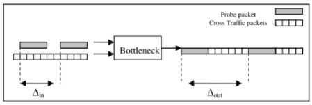
Fig.9. The Probe Gap Model for Estimating Available Bandwidth [9]

PGM assumes that all routers along the path use FIFO queuing; cross traffic follows a fluid model (i.e. crosstraffic packets have an infinitely small packet size); average rates of cross traffic change slowly and is constant for the duration of a single measurement; there is a single bottleneck which is both the narrow and tight link for that path; and finally, the capacity C of the bottleneck is known in advance.

• E.    TCP Connections and Emulation

This methodology is used to measure the throughput-related metrics (i.e. achievable throughput and BTC) by establishing either a single or several parallel TCP connection(s) to a selected host and trying to send data as fast as possible. To gain an insight into the working principle, an understanding of the TCP protocol is required. Particularly, a TCP connection starts with the slow start phase. During the slow start phase, the congestion window is doubled per RTT until the previously set threshold is reached. This threshold value can be set arbitrarily high when the connection is established. Often the value of "Advertised Windows" is used as it indicates the free space in the buffer of the receiver. Since the sender doubles the congestion window per RTT, the congestion window increases exponentially. The exponential growth of the congestion window allows a TCP connection to quickly reach the so-called equilibrium [10].

The slow start algorithm can terminate in two possible ways. Either the threshold is reached, or packet losses occur. If the threshold is reached, the congestion window is not further increased and remains constant. If packet losses occur, the threshold is reduced to half the current congestion window. From this halved place then begins the so-called congestion avoidance phase. Congestion avoidance aims to maximize the throughput while avoiding the congestion as much as possible. Therefore, in contrast to the slow-start phase, the congestion window only increases linearly from this halved point. More specifically, for each RTT, the congestion window is increased by one MSS. This procedure is referred to as "additive increase".

Tool	Metric	Methodology	Forward/ Reverse	Deployment	Layer	Active/ Passive	Protocol
Pathrate [31]	End-to-end capacity	PP	Forward	Double-ended	3	Active	UDP
PBProbe [32]	End-to-end capacity	PP	Forward and Reverse	Double-ended	3	Active	UDP
CapProbe [18]	End-to-end capacity	PP	Forward	Single-ended	3	Active	ICMP
AsymProbe [33]	End-to-end capacity	PP	Forward and Reverse	Single-Ended	3	Active	TCP
SProbe [15]	End-to-end capacity	PP	Forward and Reverse	Single-Ended	3	Active	TCP
Nettimer [4]	End-to-end capacity	PP	Forward and Reverse	On each observation point	2	Passive	Layer 2 protocol
Bprobe [34]	End-to-end capacity	PP	Forward	Single-Ended	3	Active	ICMP
PPrate [35]	End-to-end capacity	PP	Forward and Reverse	From trace file	2	Passive	TCP
Pathchar [5]	Per-hop capacity	VPS	Forward	Single-Ended	3	Active	UDP; ICMP
Clink [20]	Per-hop capacity	VPS	Forward	Single-Ended	3	Active	UDP
Pchar [36]	Per-hop capacity	VPS	Forward	Single-Ended	3	Active	UDP; ICMP

Table 2. Classification of Tools for Estimating the End-To-End Available Bandwidth

Tool	Metric	Methodology	Forward/ Reverse	Deployment	Layer	Active/ Passive	Protocol
ABwProbe [17]	End-to-end available bandwidth	PRM	Reverse	Single-ended	3	Active	TCP
Abget [16]	End-to-end available bandwidth	PRM	Reverse	Single-Ended	3	Active	TCP
Pathload [12]	End-to-end available bandwidth	PRM	Forward	Both-Ended	3	Active	UDP
Yaz [37]	End-to-end available bandwidth	PRM	Forward	Both-Ended	3	Active	UDP
ASSOLO [38]	End-to-end available bandwidth	PRM	Forward	Both-Ended	3	Active	UDP
Pathchirp [39]	End-to-end available bandwidth	PRM	Forward	Both-Ended	3	Active	UDP
Spruce [9]	End-to-end available bandwidth	PGM	Forward	Both-Ended	3	Active	UDP
IGI [40]	End-to-end available bandwidth	PGM	Forward	Both-Ended	3	Active	UDP
Delphi [41]	End-to-end available bandwidth	PGM	Forward	Both-Ended	3	Active	UDP

• A.    Challenges in Internet Environment

One of the most relevant property of an estimation tool is its resistance to cross traffic as Internet paths almost always contain cross traffic. To enhance the robustness of tools to cross traffic, several techniques have been proposed including confidence intervals [19], kernel density estimator and received/sent bandwidth ratio filtering techniques [4], minimum delay sum [18]. Unfortunately, there is no standard statistical approach that always leads to correct estimates. The main reason making the deal with the cross traffic difficult is that there exist several types of cross traffic with different behaviors (such as constant cross traffic with different rates, bursty cross traffic, self-similar cross traffic or cross traffic obeying to a distribution like Poisson or Pareto distribution etc.) that interfere with an estimation procedure in different ways. Also, hop-persistent or path-persistent cross traffic patterns influence the estimation accuracy differently.

In packet-switched networks, data packets belonging together can reach their destination over different paths. This could be caused, e.g., due to dynamic route alternation or load sharing on a measurement path. Route

Table 3. Classification of Tools for Measuring the End-To-End BTC and Achievable Throughput

Tool	Metric	Methodology	Forward/Reverse	Deployment	Layer	Active/ Passive	Protocol
Netperf [42]	End-to-end achievable throughput	Parallel TCP Connections	Forward and Reverse	Both-Ended	4	Active	UDP; TCP
Iperf [27]	End-to-end achievable throughput	Parallel TCP Connections	Forward and Reverse	Both-Ended	4	Active	UDP; TCP
Cap [43]	BTC	Emulated TCP Connection	Forward	Both-Ended	4	Active	UDP
TReno [44]	BTC	Emulated TCP Connection	Forward	Single-Ended	4	Active	ICMP

Challenges, Practical Issues and Difficulties in Estimating Bandwidth-Related Metrics

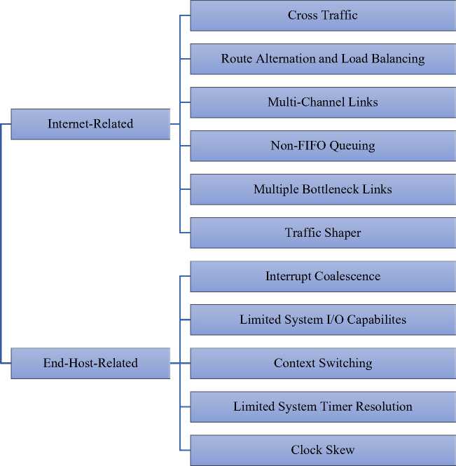
Fig.10. Overview of Classification of Challenges, Practical Issues and Difficulties Affecting the Accuracy of Estimation Techniques and Tools

alternation is the property of a path between two hosts to change over time, usually between a small set of possibilities (e.g. in case of node failures or load balancing). Note that in case of route alternation, there is only one possible route that a router can take at a given time. Contrary to route alternation, load sharing can route the packets over two or more different interfaces. Assume that on a measurement path, during the probing process such a route alternation or load sharing occurs. Then, the probe traffic will be transmitted over different links/paths which potentially will suggest different link/path characteristics (including different bandwidth speeds) causing significant estimation inaccuracies. Therefore, a robust tool should characterize the measurement path to be flexible to bandwidth and route changes. For instance, when clink [20], a hop-by-hop capacity estimation tool, encounters a routing instability, it collects data for all the paths it encounters, until one of the paths generates enough data to yield an acceptable estimate.

Along a path, a link can be multi-channeled which means that it is made up of many parallel channels. If a link of total capacity C is made up of k channels, the individual channels forward packets in parallel at a rate of C/k. In such a case, a tool may incorrectly tend to estimate the capacity of a single channel, instead of the total capacity of that link. Pathrate, e.g., uses packet trains of different lengths to detect and mitigate the effect of multi-channel bottleneck links such as ISDN links.

Several estimation methodologies and tools have the fundamental assumption that bottleneck routers use FIFO-queuing, i.e. what comes in first is handled first. Other Non-FIFO queue processing techniques such as prioritized or class-based queuing disciplines could distort the measurement process. Ideally, the estimation methodology of a tool should be independent of queuing disciplines of intermediate routers to be successfully used for deployment on Internet paths. The study in [21], e.g., proposes a technique for estimation of end-to-end available bandwidth that is independent of the network queuing discipline used by intermediate routers along a path.

The estimation technique of a robust tool should remain valid in the presence of multiple bottleneck links on a path. For example, PGM-based tools like spruce [9] assume that there is only a single bottleneck link which is both the narrow and tight link for that path. On the other side, there are also tools such as MultiQ [22] which are not only robust to multiple bottlenecks but also able to estimate the bandwidth of multiple congested bottlenecks.

In Internet, traffic shapers are often employed to control the rate of the networking traffic to guarantee some QoS parameter like latency, throughput and avoid bursty traffic. In such a scenario, the measurement process and result of a tool may be affected if its probing rate is higher than the rate the traffic shaper allows. Moreover, in case of capacity estimation, the link on which traffic shaping will be performed will have two different capacity metrics, namely the unlimited raw capacity and the sustainable rate of the traffic shaper. Thus, if a tool’s estimation methodology cannot overcome traffic shaping limitations, it should at least clearly define, which capacity metric it intends to measure for paths with traffic shaping nodes.

• B.    End-Host-Related Challenges

Interrupt coalescence (IC) is a well-known and proven technique for reducing CPU utilization when processing high packet arrival rates. Normally, a NIC without IC generates an interrupt for each incoming packet. This causes significant CPU load when packet arrival rate increases. By using IC, the workload for the host processor can be reduced significantly by grouping multiple packets, received in a short time interval, in a single interrupt. In this way, the number of interrupts to be generated will be reduced significantly. However, lower CPU utilization is done at the cost of increased network latency, since the frames are first buffered at the NIC before they are processed by the operating system (the host is not aware of the packet until the NIC generates an interrupt). Thus, the receiving timestamps for the packets sent by an estimation tool will be distorted (in such a case, all incoming packets may have the same timestamp) which may lead to erroneous estimations. To overcome IC, several tools such as IMR-Pathload [23] and ICIM [24] have been proposed, which incorporates robust IC detection algorithms to still enable reliable estimates of bandwidth metrics under a wide range of interrupt delays.

Much estimation tools fail to accurately estimate highspeed network bandwidth since they do not take the capabilities of the measurement host system into account (e.g. host’s memory, I/O bus speed etc.). If end system capabilities are involved, then the estimation will be of the end system throughput and will not indicate a correct assessment of network bandwidth [25]. Thus, either the bandwidth estimation algorithm should not be dependent on end host performance (e.g. STAB [26]) or tools should implement additional methods to determine if the end hosts can perform a proper measurement.

Most estimation tools are based on sending probing packets at a certain transmission rate, i.e. they must send packets in regular intervals to perform a proper measurement (e.g. pathload, PBProbe and abget). Consider that a tool needs to send packets at a transmission rate R with s , i.e., every t time units, a packet of size s should be sent. Two different approaches can be taken to achieve the rate R . First, a tool could perform busy waiting by continuously checking the system clock and send packets of size s every time when the clock reaches the corresponding value of t . This approach is, e.g., taken by iperf [27] tool which intrusively measures the end-to-end achievable throughput of a network path. The maximum rate R obtainable with this approach depends on the time which is required to perform the clock checking process. Though the busy waiting mechanism allows achieving high transmission rates, it wastes a lot of CPU cycles affecting the efficient processing of tasks from other applications, especially if the measurement process lasts for several seconds which is typically the case for most of the tools.

In the second approach, an estimation tool associates its action of sending probing packets with a system timer mechanism which is a recurring timeout process in an OS. Every time when this timer expires, and a timeout occurs, the tool fires its probing packets. Consequently, creating a timeout event which sends packets of size s with timeout value as t allows achieving the rate R . This approach avoids the problem of busy waiting since the CPU is merely stressed if and only if a probing packet should be sent. Due to this significant advantage, almost all tools use this timing mechanism. Unfortunately, contrary to busy waiting mechanism, the maximum transmission rate obtainable using this approach is strongly limited by the insufficient system timer resolution. The current minimum system timer resolution among the common operating systems is 1 µs. By considering the biggest size of 1500 Byte in classic Ethernet networks, only a transmission rate of R = 1.2 Mb/s can be achieved. To overcome this problem, the technique of packet trains is proposed. For further information, we refer the reader to the respective publications [14]. Note that a clock’s resolution also affects the preciseness of packet timestamps. The higher the clock’s resolution is, the more accurate the timestamp on the packets.

Another challenge arises when a tool’s measurement process gets interrupted by a context switch at the end hosts. Assume that a probing stream with a specified rate is transmitted by an end host, i.e. the probe packets are sent out periodically every time unit. If during this transmission process a context switch occurs, the specified rate can’t be sustained any more reducing the estimation accuracy. Thus, to avoid this problem, a tool should either detect the occurrence of context switching or select the transmission period of its probing stream as short as possible to complete before a context switch interruption occurs. DIChirp [28] is, e.g., an end-to-end available bandwidth estimation tool which is designed to minimize the impact of a context switching during a measurement session.

Several both-ended tools rely on the assumption of a synchronized clock between the endpoints. However, the clocks on different machines are usually not synchronized and the offset between two different clocks usually changes over time. To ensure reasonable estimation accuracy, a tool should be robust to this clock skew problem. Examples of tools that do not require any clock synchronization between measurement hosts are Forecaster [29] and Pathvar [30].

• VI. Conclusion

In principle, in bandwidth estimation research there are three popular metrics: capacity, available bandwidth and throughput. PP measures the end-to-end capacity of a path between two hosts. In other words, the maximum bandwidth of the weakest link on the entire path between two hosts is estimated. The disturbance of the normal network traffic caused by PP is relatively small, since few packets are sufficient for a good estimate and the probing duration is independent of the number of hops passed through. VPS associates the RTTs with several packets of different sizes. The capacity of each individual hop from a sender to a receiver is estimated. The disadvantages of this technique are that the total duration of the measurement is very high, and the generated measurement traffic increases linearly with respect to the number of hops measured. The basic idea in PRM is that the OWDs of a periodic packet stream show an increasing trend when the stream’s rate is higher than the available bandwidth between two hosts. Each stream rate tested requires a large amount of data, but the short duration of each burst does not interfere with competing traffic. Another alternative end-to-end available bandwidth estimation technique is PGM which is characterized by its lightweight and fast estimation procedure. Compared to PRM that require multiple iterations with different probing rates, PGM uses a single probing rate and it infers the available bandwidth from a direct relation between the input and output rates of measurement packet pairs. Finally, throughput can, in turn, be divided into achievable throughput and BTC. Both metrics are measured by actively overloading TCP connections between two hosts. Despite the highest level of measurement accuracy, this technique has the demerit that it saturates the path, significantly increases the delays and jitter, and potentially causes losses to other TCP flows. In addition to the estimation techniques presented in this study, there are several other methodologies that were proposed and implemented in the related literature. It can be concluded that each methodology exhibits its own advantages and disadvantages, and there is no generalizable superiority of one estimation technique over the others that consistently performs well over all network settings, scenarios and conditions.

The best decision about the selection of the more appropriated tool depends on both the network environment on which they are later deployed and their use cases. Tools to be deployed on real Internet paths must be able to cope with asymmetric links. Moreover, due to limited access to the remote Internet hosts, use of single-ended tools is needed which are only deployed locally on the user’s host without requiring the cooperation from the other end of a measurement path. However, for large scale studies of Internet path characteristics, active tools become difficult because of the probe overhead they cause and the need to be deployed on each measurement host. In such cases, passive tools demonstrate their benefits which can be flexibly placed at a few appropriate observation points to capture and analyze the passing real traffic. In case of only a few interesting paths where the user has access to both the sender and receiver hosts, active and doubleended tools are more suitable since in general, they achieve more accurate results than single-ended or passive tools. Estimations in wireless networks, on the other hand, require non-intrusive and lightweight estimation procedures with fast convergence times whereas use cases such as dynamic server selection or congestion control support require tools that can produce quick real-time estimations.

Finally, despite the significant previous research on estimating bandwidth-related metrics, it can be concluded that up to now the research community is still rather far from having consistently accurate and robust tool implementations. The broad survey revealed that there are a variety of different challenges, practical issues and difficulties that can negatively affect an estimation procedure and lead to significant estimation errors. Such challenges range from typical Internet-related issues such as cross traffic disturbances, route alternations, multichannel and asymmetric links, traffic shapers or network components working with non-FIFO queuing disciplines to end-host related challenges such as NIC's IC mode, OS's limited system timer resolution, limited end-system capabilities and the context switching problem. Thus, to have the capability to be deployed under real environments with such network settings, a well-established estimation technique should consider these issues in its design and implementation phase. Consideration in that context means that it should either attempt to overcome such issues to still give acceptable accurate estimates or detect such inconveniences and abort the estimation process instead of reporting a potentially inaccurate estimate.

This work is supported by Adana Science and Technology University Scientific Research Projects Center under grant no 18103001.

• [1]     R. Prosad et al. , “Bandwidth estimation: metrics,

  measurement techniques, and tools,” IEEE Netw. , vol. 17, no. 6, pp. 27–35, 2003.

• [2]    C. D. Guerrero and M. A. Labrador, “On the

  applicability of available bandwidth estimation techniques and tools,” Comput. Commun. , vol. 33, no. 1, pp. 11–22, 2010.

• [3]    A. S. Sairam, “Survey of Bandwidth Estimation

  Techniques,” Wirel. Pers. Commun., vol. 83, no. 2, pp. 1425–1476, 2015.

• [4]    K. Lai and M. Baker, “Nettimer: A tool for measuring

  bottleneck link bandwidth,” in Proceedings of the USENIX Symposium on Internet Technologies and Systems , 2001, vol. 134, pp. 1–12.

• [5]    A. B. Downey, “Using pathchar to estimate Internet link

  characteristics,” ACM SIGCOMM Comput. Commun. Rev. , vol. 29, no. 4, pp. 241–250, 1999.

• [6]     X. Su, X. Yan, and C.-L. Tsai, “Linear regression,”

Wiley Interdiscip. Rev. Comput. Stat. , vol. 4, no. 3, pp. 275–294, 2012.

• [7]    R. S. Prasad, C. Dovrolis, and B. A. Mah, “The effect of

  layer-2 switches on pathchar-like tools,” Proc. Second ACM SIGCOMM Work. Internet Meas. - IMW ’02 , no. 5, p. 321, 2002.

• [8]     V. Paxson, “End-to-end routing behavior in the internet,”

IEEE/ACM Trans. Netw. , vol. 5, no. 5, pp. 601–615, 1997.

• [9]    J. Strauss, D. Katabi, and F. Kaashoek, “A measurement

  study of available bandwidth estimation tools,” in Proceedings of the ACM SIGCOMM Internet Measurement Conference, IMC , 2003, pp. 39–44.

• [10]    A. O. Tang, J. Wang, S. Hegde, and S. H. Low, “Equilibrium and fairness of networks shared by TCP Reno and Vegas/FAST,” Telecommun. Syst. , vol. 30, no.

4 SPEC. ISS., pp. 417–439, 2005.

• [11]    F. Abut, “Towards a Generic Classification and Evaluation Scheme for Bandwidth Measurement Tools,” Signals Telecommun. J. , vol. 1, pp. 78–88, 2012.

• [12]    M. Jain and C. Dovrolis, “Pathload: a measurement tool for end-to-end available bandwidth,” in Proceedings of the Passive and Active Measurements (PAM) Workshop , 2002, pp. 1–12.

• [13]    K. Harfoush, A. Bestavros, and J. Byers, “Measuring capacity bandwidth of targeted path segments,” IEEE/ACM Trans. Netw. , vol. 17, no. 1, pp. 80–92, 2009.

• [14]    C. Dovrolis, P. Ramanathan, and D. Moore, “What do packet dispersion techniques measure?,” in Proceedings of IEEE INFOCOM , vol. 2, pp. 905–914, 2001.

• [15]    S. Saroiu, P. Gummadi, and S. Gribble, “Sprobe: A fast technique for measuring bottleneck bandwidth in uncooperative environments,” in Proceedings of IEEE INFOCOM , pp. 1–11, 2002.

• [16]    D. Antoniades, M. Athanatos, and A. Papadogiannakis, “Available bandwidth measurement as simple as running wget,” in Proceedings of Passive and Active Measurements Conference (PAM) , 2006, pp. 61–70.

• [17]    D. Croce, T. En-Najjary, G. Urvoy-Keller, and E. W.

  
  

  Biersack, “Non-cooperative available bandwidth estimation towards ADSL links,” in Proceedings of IEEE INFOCOM , 2008.

R. Kapoor, L. Chen, and M. Gerla, “CapProbe: A Simple and Accurate Capacity Estimation Technique,” in SIGCOMM ’04 Proceedings of the 2004 conference on Applications, technologies, architectures, and protocols for computer communications , 2004, pp. 67– 68.

C. L. T. Man, G. Hasegawa, and M. Murata, “An Inline measurement method for capacity of end-to-end network path,” in 3rd IEEE/IFIP Workshop on End-to-End Monitoring Techniques and Services, E2EMON , 2005, vol. 2005, pp. 56–70.

A. B. Downey, “Clink,” 1999. [Online]. Available:

M. Kazantzidis, D. Maggiorini, and M. Gerla, “Network independent available bandwidth sampling and measurement,” Lect. NOTES Comput. Sci. , vol. 2601, pp. 117–130, 2003.

S. Katti, D. Katabi, C. Blake, E. Kohler, and J. Strauss, “MultiQ: automated detection of multiple bottleneck capacities along a path,” IMC ’04 Proc. 4th ACM SIGCOMM Conf. Internet Meas. , pp. 245–250, 2004.

S. R. Kang and D. Loguinov, “IMR-Pathload: Robust available bandwidth estimation under end-host interrupt delay,” in Lecture Notes in Computer Science , 2008, vol. 4979 LNCS, pp. 172–181.

C. L. T. Man, G. Hasegawa, and M. Murata, “ICIM: An Inline Network Measurement Mechanism for Highspeed Networks,” in 2006 4th IEEE/IFIP Workshop on End-to-End Monitoring Techniques and Services , 2006, pp. 66–73.

G. Jin and B. L. Tierney, “System Capability Effects on Algorithms for Network Bandwidth Measurement,” in Proceedings of 3rd ACM SIGCOMM Conf. Internet Meas. , pp. 27–38, 2003.

V. J. Ribeiro, R. H. Riedi, R. G. Baraniuk, and J. Navratil, “Spatio-temporal available bandwidth estimation for high-speed networks,” in ISMA 2003 Bandwidth Estimation Workshop , 2003, pp. 6–8.

A. Tirumala, L. Cottrell, and T. Dunigan, “Measuring end-to-end bandwidth with Iperf using Web100,” in Proceedings of Passiv. Act. Meas. Work., pp. 1–8, 2003.

Y. Ozturk and M. Kulkarni, “DIChirp: Direct injection bandwidth estimation,” Int. J. Netw. Manag. , vol. 18, no. 5, pp. 377–394, 2008.

M. Neginhal, K. Harfoush, and H. Perros, “Measuring Bandwidth Signatures of Network Paths,” Network , pp. 1–12, 2007.

M. Jain and C. Dovrolis, “End-to-end estimation of the available bandwidth variation range,” ACM SIGMETRICS Perform. Eval. Rev. , vol. 33, no. 1, p. 265, 2005.

C. Dovrolis, P. Ramanathan, and D. Moore, “Packetdispersion techniques and a capacity-estimation methodology,” IEEE/ACM Trans. Netw. , vol. 12, no. 6, pp. 963–977, 2004.

L.-J. J. Chen, T.Sun, B.-C. C. Wang, M. Y. Y. Sanadidi, and M. Gerla, PBProbe: A capacity estimation tool for high speed networks , vol. 31, no. 17. 2008.

L. Chen, T. Sun, G. Yang, M. Y. Sanadidi, and M. Gerla, “End-to-End Asymmetric Link Capacity Estimation,” in IFIP Networking , 2005, pp. 780–791.

R. L. Carter and M. E. Crovella, “Dynamic server selection using bandwidth probing in wide-area networks,” in Proceedings of IEEE INFOCOM, 1997.

• [35]    T. En-Najjary and G. Urvoy-Keller, “PPrate: A Passive Capacity Estimation Tool,” in 2006 4th IEEE/IFIP Workshop on End-to-End Monitoring Techniques and Services , 2006, pp. 82–89.

• [36]    B. A. Mah, “pchar: A Tool for Measuring Internet Path Characteristics,”     2001.     [Online].     Available:

˜bmah/Software/pchar/.

• [37]    J. Sommers, P. Barford, and W. Willinger, “Laboratorybased calibration of available bandwidth estimation tools,” Microprocess. Microsyst. , vol. 31, no. 4 SPEC. ISS., pp. 222–235, 2007.

• [38]    E. Goldoni, G. Rossi, and A. Torelli, “Assolo, a New Method for Available Bandwidth Estimation,” 2009 Fourth Int. Conf. Internet Monit. Prot. , pp. 130–136, 2009.

• [39]    M. Ładyga, R. H. Riedi, R. G. Baraniuk, J. Navratil, and L. Cottrell, “pathChirp: Efficient Available Bandwidth Estimation for Network Paths,” in Passive and Active Measurement Workshop , 2003.

• [40]    N. Hu and P. Steenkiste, “Evaluation and characterization of available bandwidth probing techniques,” IEEE J. Sel. Areas Commun. , vol. 21, no. 6, pp. 879–894, 2003.

• [41]    V. Ribeiro, M. Coates, R. Riedi, S. Sarvotham, B. Hendricks, and R. Baraniuk, “Multifractal cross-traffic estimation,” ITC Spec. Semin. IP Traffic Meas. , pp. 1– 15, 2000.

• [42]    “Netperf Homepage,” 2018. [Online]. Available: https://hewlettpackard.github.io/netperf/ .

• [43]    M. Allman, “Measuring end-to-end bulk transfer capacity,” Proc. First ACM SIGCOMM Work. Internet Meas. Work. - IMW ’01 , no. November, p. 139, 2001.

• [44]    M. Mathis and J. Mahdav, “Diagnosing internet congestion with a transport layer performance tool,” in INET’96 , 1996.