Tomographic Convex Time-Frequency Analysis

In this paper, we propose a method to compute Chambolle Pock’s algorithm. This algorithm is efficient to solve a deblurring problem in tomography.

We aim to solve a problem of image restoration dealing with Positron emission tomography (PET). Our goal is to reduce the dose of radioactive drug given to the patient in PET scan and to get a non blurred image. With high dimensions, we want to find the representative components of the image. So, we take an image with some known, or estimated degradation and we restore it to its original appearance.

In order to reduce the noise, we have to minimize a functional in our case dealing with Poisson noise. Then, we have to solve a linear inverse problem.

Nesterov proposes the gradient method as cited in [1], Combettes and Wajs propose a proximal forwardbackward splitting algorithm as cited in [2].

Beck and Teboulle, propose a fast iterative thresholding algorithm as cited in [3]. Daubechies et al propose an interative thresholding algorithm with a sparsity constraint as cited in [4]. And Chambolle Pock propose a first-order primal-dual algorithm as cited in [5]. We show that Chambolle Pock’s algorithm is the most suitable for resolving our problem after comparing the algorithms cited above. Also, we give an explicit form of its variables. We present four algorithms related to Chambolle Pock’s algorithm:

Dupé et al propose a fast iterative forward backward splitting algorithm as cited in [6]. Moreau describes the duality in a Hilbert Space in [7]. Figueiredo and Nowak propose an expectation –maximization algorithm for Image Restoration based on a penalized likelihood formulated in the wavelet domain in [8]. Cohen et al propose numerical methods for the treatment of inverse problems based on adaptative wavelet Galerkin dicretization in [9].

We describe five algorithms proposed to get a well-qualified image, compared to the PSNR value: Nain et al propose the Peer Group Average algorithm as cited in [10]. Jiang et al propose the Stationary wavelet transform algorithm as cited in [11]. Mahmoud et al propose the Log Gabor filter as cited in [12]. Raj and Venkareswall propose the double density dual tree comp as cited in [13] and they propose the Split Bregman, total variation as cited in [14]. Zanella et al propose the scaled projected gradient method as cited in [15]. We explain the PET technique and formulate the problem.

In medical imaging, (PET) is a gamma imaging technique that uses radio tracers that emit positrons, the antimatter counterparts of electrons. In PET the gamma rays used for imaging are produced when a positron meets an electron inside the patient's body, an encounter that annihilates both electron and positron and produces two gamma rays traveling in opposite directions. By mapping gamma rays that arrive at the same time, the PET system is able to produce an image with high spatial resolution.

Our problem can be formulated as

Rf = p (1)

Where: R e M (R " , R ™ ) is the projection matrix R_u represents the weight of pixel j in the ray of projection i . f e R " the image to reconstruct. And p e R ™ the whole projections obtained in several directions or the sinogram, a radiograph to visualize any abnormal opening in the body, following the injection of contrast media into the opening.

The remainder of the paper is organized as follows. In section II , a review of the necessary related work required to effectively implement our algorithm is presented for convex problems. The method and how we will compute our proposed algorithm is described in

Section Ш . After that, application of the proposed algorithm and results is discussed in section IV, and we draw our conclusion in the last section.

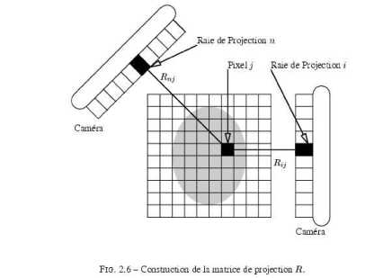
Fig.1. Construction of the projection matrix R .

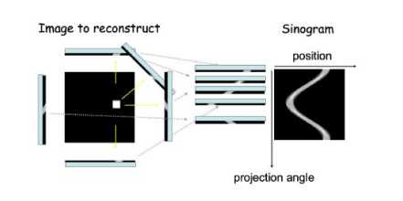
Fig.2. Sinogram obtained after the projections over the image to reconstruct

• II.  Related Work

• A.    Gradient Method

The gradient method is to minimize a convex differentiable function f . This method consists on backtracking lines search. And each line search minimizes f ( x - t V f ( x ) ) over t . Every iteration is inexpensive and it doesn’t require second derivatives. Newton's method also minimize a convex differentiable function, uses the first few terms of the Taylor series of a function f ( x ) in the vicinity of a suspected root.

The conjugate gradient method can be used to solve unconstrained optimization problems like the gradient method. It is a descent method.

The subgradient method is an algorithm for minimizing a non differentiable convex function. It is not a descent method; the function value can often increase.

Solving min ( F ( x ) + G ( x ) ) = min f ( x )      (2)

xeX V                7    xeX where F: X ^ R is a L -lipschitz differentiable function and G: X ^ R is a convex function non differentiable, requires the proximity operator as defined below. The operator proxG : X^ X

. (             1           2

x ^ arg min I G ( y ) + — | x - y| y e X  V        2

is called proximity operator associated to G . As cited in [2] and [3]. If G is differentiable, the subgradient projection method gives the solution. As cited in [1]. This method converges slowly, and the rate of convergence is 1 _k

The projected subgradient method is similar to the subgradient method, we consider a convex set.

• B.    Extension of the Gradient Method

We will discuss two methods:ISTA, Iterative Shrinkage-Thresholding Algorithm and FISTA, Fast Iterative Shrinkage-Thresholding Algorithm, as cited in [3] and [4]. These methods are the extension of the gradient method.

ISTA consists on constructing on each iteration a regularization of linear differentiable functions. It means making some descent of gradient on F differentiable and computing the proximity operator on the non differentiable G .

FISTA is an accelerated version of ISTA. Chambolle Pock [5] show that solving the following problem min F(Kx) + G(x) which is the sum of two convex xeX functions, lower semi-continuous non differentiable with X, Y two finite spaces holding the scalar product. K: X ^ Y linear continuous operator with the inducted norm

K

max

{ x e X with || x ||<1 }

Kx

requires this convergent algorithm while _to\ K ²|| <  1.

Initialization Choose to > 0, 9 e [ 0,1 ]    ( x °, y ⁰ ) e X x Y

and x0 = x0

y n ^{+ 1} = prox _{a F} . ( y n + CT Kx" )

< xn+1 = proxTG (xn -tK*yn+1)         (5)

xn+1 = xn+1 + 9 (xn+1 - xn)

While taking

9 = 0                     (6)

in that algorithm we obtain the speed of convergence approximately of (1 N ). We can improve the rate of convergence to (^ N ²). We summarize the algorithms their criteria and their rate of convergence on the table below.

Table1. Comparative table of iterative methods

Method	Criteria	Rate of convergence
Gradient method	f convex, L -Lipschitz continuously differentiable	c ( 1 - q ) k
Newton method	f convex, L - Lipschitz continuously differentiable	c (1 - q )2 k
Conjugate gradient method	f convex, L -Lipschitz differentiable	Not better than the gradient method
Subgradient method	f convex non differentiable	Slower than the Newton method
ISTA	f , g convex functions f L -lipschitz differentiable g possibly non smooth	1 k
MTWIST Monotone version of TWIST(Two step ISTA for extremely ill-conditioned problems)	f , g convex functions f L -lipschitz differentiable g possibly non smooth	У 5 r (k ) 5 Ук 2
FISTA	f , g convex functions f L -lipschitz differentiable g possibly non smooth	1 k 2
Projected subgradient method	f convex non differentiable, X E C a convex set	Not better than 1 k
Chambolle Pock’s algorithm	f , g lower semi-continuous conjugate convex functions	Can be accelerated to 1      if k 2 f * or g is uniformly convex.

In[6] they present a deconvolution algorithm, fast iterative thresholding algorithm, taking into consideration the Poisson noise. For denoising the images, they use the Anscombe transform. And finally, they select the regularizing parameter by using the generalized cross validation based model selection. They recommend using sparse-domain regularization in many deconvolution applications with Poisson noise.

In [7], Moreau propose dual functions and conjugate functions in the Hilbert space. He talks about proximity operator.

In [8], they propose a wavelet-based criterion for

Image Deconvolution. This algorithm MPLE/ MAP criterion maximum penalized likelihood estimator, maximum a posteriori alternates between Fourier domain filtering and wavelet domain denoising.

In [9], they propose Galerkin methods for inverse problems based on wavelets. They combine a thresholding algorithm on the data with a Galerkin inversion on a fixed linear space and then they invert by constructing a smaller space adapted to the solution iteratively constructed.

In [10], many mixed noise removal techniques were compared such as Peer Group Averaging (PGA), Vector Median Filter (VMF), Vector Direction Filter (VDF), Fuzzy Peer Group Averaging (PGA), and Fuzzy Vector Median Filter (FVMF). (PGA) is a non-linear filter, whose aim is to average over a peer group rather than the whole window. (FVMF) performs a weighted averaging where the weight of each pixel is computed according to its similarity to the robust vector median. They prove that (PGA) is advisable when the image size is small and if the image size is large it is better to use (FVMF). Also, (PGA) gives best visual quality results while (FVMF) gives the worst visual quality results.

In [11], they develop a novel method to improve the Visual quality of X-ray CR images, consisting of a wavelet-based filter denoising based on SWT:Stationary Wavelet Transform and the wavelet thresholding then, they enhance the image contrast using Gamma Correction and after extract and classificate high frequency components into three feature images and then Image fusion obtained after adjusting the compression ratio of non-diagnosis feature component in the high signal range and calibrate the parameter.

In [12], they show that the Log Gabor Filter, a filter in the transform domain gives good images quality, PSNR values and CPU time, while Speckle Reducing Anisotropic Diffusion (SRAD) a spatial filtering is better than several commonly used filters including Gaussian, Gabor, Lee, Frost, Kuan, Weiner, Median, Visushrink, Sureshink and also the Homorphic Filter, but on the other hand, has a very high CPU compared to the other filters.

In [13], they show that in order to remove the noise of Poisson and Rician from medical images, the double density dual tree complex wavelet transform based on discrete wavelet transform is performing based on discrete wavelet transform is performing well than the other transforms.

In [14], they show that total variation based regularization split Bregman method from optimization method is well-suited to image restoration in medical images and it is better than the traditional spatial domain filtering methods.

In [15], they show that for Poisson noise removal the scaled gradient projection method based on a Bayesian approach is more efficient than the gradient projection methods.

• III.    Method And The Proposed Algorithm

The process of image construction is f : isotopes j concentration on pixel j, fj > 0 . Ry : the average number of photons detected on i per unit of isotopes concentrations on pixel j . We note p, = Z",=1 Rf              (7)

In fact, what we measure on each pixel i , is the realization of a random variable p>=XZ j eK -Rf         (8)

of Poisson parameter p . One way of finding f is to estimate the maximum of likelihood.

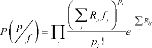
All p are independent. (And n are random variables). The maximum of likelihood estimate is the value that makes the observed data the most probable. Rather than maximizing this product, we often use the fact, that the logarithm is an increasing function so it will be equivalent to maximize the log likelihood. Maximizing likelihood on f means minimizing the criteria:

J (. f ) = Z Z ^R , f,-piog Z Rf

i of spatially invariant blurs represents a two-dimensional convolution operator. The problem of estimating x from the observed blurred and noisy image p is called an image deblurring problem.

The blur operator is unbounded, we are in ill-posed problems. The generalized inverse operator may be unbounded. So, it has to be replaced by bounded approximants, so that numerically stable solutions can be defined and used as meaningful approximations of the true solution corresponding to the exact data. This is the purpose of regularization.

In image deblurring applications, R is chosen as R = AW , where A is the blurring matrix and W contains a wavelet basis. R corresponds to performing inverse wavelet transform. We deal with the l norm regularization criterion because most images have a sparse representation in the wavelet domain. In our case, we are using medical data represented by photon images degraded by Poisson noise. Because of this, it is a difficult task to remove the noise. However, if we can remove Poisson noise effectively, we will acquire a fine image from the degraded image produced with a small amount of photons. This may lead to a reduction of the probability of not only medical exposure, but also medical errors. To accomplish the effective reduction of Poisson noise, the techniques based on wavelet transform have been proposed recently. The method gives thresholding in each wavelet domain, maintaining the features of an original signal. As seen in the related work, Chambolle Pock’s algorithm requires less properties than the other algorithms.

We will choose to minimize F ( K x ) + G ( x )

Where F ( K x ) = J ( x ) , K = R and G is non differentiable. F and G are lower semi-continuous convex functions.

• B.    Choice Of The Functionals

We will minimize it under the constraint: f e IR+ .

n

We have to minimize the error. This functional is convex but not differentiable on IR+, so if she takes a minimum, this minimum is global. J takes a global minimum, in this case, it is not unique because R is not invertible on prior. It is an ill-posed inverse problem.

• A. Explanation of a basic linear inverse problem

A basic linear inverse problem leads us to study a discrete linear system of the form:

R x = p + w              (11)

where R e R ^{m x} " and p e IR. ^m are known, w is an unknown noise and x is the “ true’’ and unknown image to be estimated. In image blurring problems, p e IR. ^m represents the blurred image. In these applications, the matrix R describes the blur operator, which in the case

J ( x ) = Z

i

Z Riyxj ^- plog T Rixj

. j                       V j

is the function indicator of a

C = { x : x >  0} . _л. ( x ) =(O if

I ^

IIxlL,w =ZZI< x,^j,k >1 jk convex set x e C and else.

G ( ^x ) = C ( ( ^x ) + ^| x |^, W        (13)

We include on G the positive constraint and the wavelet l -regularization. G is the functional representing the denoising. The parameter X is the regularization parameter, which is used to control the degree of regularization.

C. Application On Chambolle Pock’s Algorithm

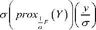
After choosing F and G convex functions as defined above, we compute: ° f *, prox^ . ( x ) and prox_TG ( x ). The prox have an explicit form. Knowing p >  0. After computing, we get:

because we know the explicit form F ( y )?.

p^rox ° F * ⁽ У ) = ^- [ y + ¹

—

prox_TG ( x ) is the projection on a positive set of inverse wavelet transform of a threshold of parameter Xt of the wavelet transform on x .

У = prox ° F	( у )
■ II У — У |r^z X = arg min -----— + F ( y ) y       2 °
= arg min y	II y — у |Г              ( х                   (23) 11 +( У p log ( x ) ,1> + Хс ( x ) 2 °
= arg min y	X ( i ,/' + f ( у ) +4 ( у ) L   2 °
= arg min y	( У‘. у ) + f ( y , )+4 ( у , )] (   2 °                   j

Differentiating f ( y ) with respect to y. , we get:

prox T G ⁽ x ) = П C [ ^{W — 1 S} ( ^W x ) ]      ⁽¹⁵⁾

• C.    Computing prox . ( y )

F (y)=X (y.— p.log( y)+^ ( У ))

x = proxCTF •< y)

f ( У )

——— = 1--L then, we have dУ i

(ухУ!+1 _ p = о

° у,2 — у,( у—°)—p ° =0

у , °

Then,

By calculating the discriminant of this binomial

x

У, + ^{1 —} V( у . ^— 1 ) 2 + ^4ctp.

А = ( у — 0 ) 2 + 4 p ,о >  0        (25)

In our case, p . >  0 .

Proof:

fi ( y i ) = y i ^— p , log⁽ У ) ⁺ АУ ( y , )      ⁽¹⁹⁾

f is lower semi-continuous over R because p. >  0

Then, f (y )=X f (x)          (20)

i delta being positive, admits two solutions:

( у ^{— о} )^—У( у ^— ° ) ² + ⁴ p °

(у—°)+7(у—°)2+4 p° у,2 =--------—:----------

We choose the second solution because for this value we get the minimum value of the prox . After Moreau’s identity, we have:

is convex lower semi-continuous over ⁿ .

For computing prox ( y ) , we will use Moreau’s identity see [7].

p ^rox ° F * ( У ) = У ^—

x, = У , ^— °

x

I

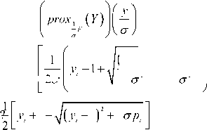
2 °

⁽ у, ^{— 1 ) 2} , ⁴°p,

Then, we will have to compute

У = prox ^ F ( у ) with ° = —

°

And we get the result.

• D.    Computing prox_TG ( x )

  Before computing proX_TG ( x ) , we aim to minimize this following functional which will help us to compute prOX _T G ( x ) .

  
  

  arg min

  a

  
  
  
  

  X у_кф_к ^— X ^a k ^ k ^{+ X} H L

  kk

  
  

  J ( a ) = || у - А Ц ² + Х Щ      (29)

  Because,

  
  

  = arg min

  a

  
  

  XI у к — a k l

  k

  
  
  
  
  

  ⁽ у_к )

  
  

  ^{+ X} I H 1

  
  
  
  

K = arg min I G (у) + — ||x - у||X I уe X V        2т/

= arg min I Xc (у ) + ЯIW\|, + — ||x — y|X у e X  V

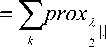
E. Computing prox^ ( у_к )

J (ak ) = | ук — ak |2 + X|ak|

We notice that this functional is convex being the sum of two convex functionals. In fact, let us compute the differential of ||y — Aa|| ■

J , ( a ) = || y — A a ||² = < У - A a ,У — A a)   (³¹)

J ( a + h ) — J ( a )

= < у — A ( a + h ) , у — A ( a + h ) )

— <  у — A a , у — A a )

= < у — A a — Ah , у — A a — Ah}

— < у — A a , у — A a )

= < у — A a , у — A a ) — < у — A a , Ah )

— < Ah , у — A a ) + < Ah , Ah ) — < у — A a , у — A a )

= — 2 < h , A ( у — A a ) ) + <  Ah , Ah )

VJ (a) = —2A* (у — Aa)

J" (a) = 2AA*

Then, J ( a ) is convex. For || a ||j we have

IXa + (1 — Я)4 ^ ЯМI, +(1 — X)|aiI, which shows that ||a|| is convex. Therefore, J (a) being the sum of two convex functions is convex. We know that J is convex, 0 edJ(x) is equivalent to say that x is the minimizer of J . Then, the minimum is reached.

Another writing of:

arg min || у — A ^ |'^:+ я a l          (36)

a

We take: у = ^уk^ and Aa = ^0t^t Then (36) kk becomes:

We compute the subgradient of J on a point a_k . And we calculate at which condition 0 ed J ( a ) .Let us consider these cases:

First case: J differentiable on a_k <  0 . We have

S J ( a k ) = { V J ( a k ) }               (39)

^{V J (a} k ) = ^{— 2 (} у к — ^a k ^{) — X}

V J ( a k ) = 0 ^— 2 у к — X = —2a_k     (40)

X Then, a, = у , + — kk ₂

The critical point is:

X „ ak = ук +-< 0           (41)

and this impose the following condition:

X .

у + — <  0

k ₂

Second case: J is differentiable on a >  0 ■

We have az (ak ) = {VJ (ak)}        (42)

we have

^{J (a} k ) = | у к ^{— a} k |^{2 + X} ^ k l

^{V J (a} k ) = ^{— 2 (} у к ^{— a} k ^{) + X}

V J ( a k ) = 0 ^— 2 у_к + X = — 2a_k   ⁽⁴³⁾

X ak = у* — 2

The critical point is

X ^a к = У к "             ⁽⁴⁴⁾

and this impose y ^ >  ^X knowing that a >  0 . In both cases, J ^(a k ) is differentiable.

Third case: a_k = 0

J is not differentiable. Let us calculate the subgradien ton 0. J (0) = |yk |2              (45)

If p ed J (0) , we get:

V A , J ( в к )-l у . 2 X p , в к >

I У к - в к\ ² -I У к Г + Дв к\ >< p , в к >   ₍₄₆₎

в к - 2 А у . + ^в кХ >< Р , в к > в к - в к ( 2 У + Р ) + ^Х|А | >

First case: Д >  0

А - А ( 2 У к + Р - X ) > 0

в к [ в к - ( 2 у . + Р - х ) ] > 0, VA .

We must have: 2 y_k + p - X <  0

Then, p < X - 2y k                (47)

Second case: А <  0

в , ¹- в к ( 2 У к + p + X ) > 0

в к [ в к - ( 2 У + p + X ) ] > 0

We must have: 2 y ^ + p + X >  0

Then, p > - X - 2 y_k

Then, we must have:

- X - 2 У к <  p <  X - 2 У к        (48)

Conclusion:

d J ( 0 ) = { a : a = - 2 y + X s , s e [ - 1,1 ]}      (49)

Then,

	f      X       2 у к - - if у к > -
proxX . ,( У к ) = < .	0 if У |< X        (50)

X;

^y к ⁺ "if ^y к <^--

Notations:

Let us note by: y the norm of y on the wavelets basis. We will design by Wy the wavelet transform y . And we will note by

G ( x ) = 1 ^ 4            (51)

The thresholding operator S is defined by:

S x ( x ) =

x - X if x >  X

0 if | x | <  X x + X if x <- X

The previous functional is a thresholding of a parameter on y . We aim to compute

К = prox_TG ( x ) .            (53)

We have:

G ( У ) = X ( У ) + ^X l| y | L y

= kV _r ⁽ У ^{) +} / У y. V j, >|       (54)

j ,

= -A- ( у )+ ^X l У^у I

Then,

К = arg min | G (y ) + 1- ||x - y|| ye X  V        2т7

= arg min [Xc (y) + X |yy\[ + ^ ||x - y|IX | ye X  V                    2т7

= arg min | Xc ( y) + X |^y|[ + ^ |^x - Уу|X ye X  V

= arg min (Xc ( Wz) + XI|z|[ + ^ ||yx - z|IX ze X   V

= n[ ^W -1 S X, (Wx ) ]

C

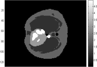
• IV. Application on Pet and results

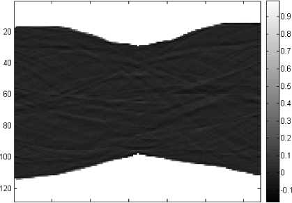
To verify the performance of the proposed algorithm, we experiment with medical images. The first three images represent the simulated data ( f , p and p ) . In the fourth and fifth images, we show results of Chambolle Pock’s algorithm after 50 iterations with о = т = 0.05 , X = 0.5 and 0 =0 .

The fourth image represents the constructed image x n ⁺ 1 in Chambolle Pock’s algorithm. And the fifth image represents the sinogram obtained y n ^{+ 1} in Chambolle Pock’s algorithm.

In the section method, by computing prox^ _f* ( y ) and prox_TG ( x ) , we removed the Poisson noise on the blurred projection operator and we get the unblurred image. Also, we get an explicit form of the parameters of Chambolle Pock’s algorithm easy to implement in matlab.

20        40 eo 80        100       120

Fig.3. Image f to reconstruct ( unknown of the algorithm).

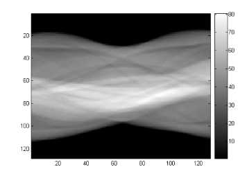
Fig.4. Image of the non blurred sinogram p .

X 40      60      80      100     120

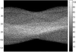
Fig.5. Image of the blurred sinogram p

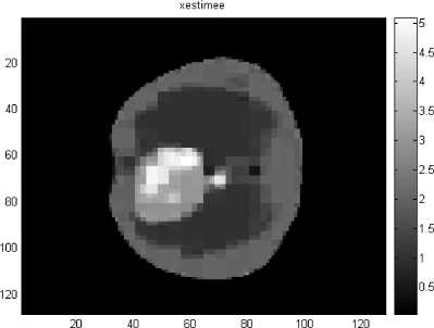
Fig.6. Image x estimation of f after 50 iterations of the algorithm.

у estimee

20        40        60        80       100      120

Fig.7. Image y after 50 iterations of the algorithm.

• V.    Conclusion

This study proposes a method to compute Chambolle Pock’s algorithm, used to solve a deblurring problem in tomography, dealing with two convex, lower semi-continuous functions. After introducing the wavelet l -regularization on the functional representing the denoising, we compute the proximity operator associated to the functions in Chambolle Pock’s algorithm and we get an explicit form of the parameters easy to implement on matlab.

The experiment results show that after computing 50 iterations of Chambolle Pock’s algorithm with ст = т = 0.05 we get an unblurred image. This algorithm is efficient in removing Poisson noise from a tomographic image.

For the future work, this research will be extended further by involving other components of other related algorithms and we expect to get better results.

Acknowledgment

This paper is fully supported by the Computer Science and Statistics Department of the Lebanese University, Fanar.