Towards Modeling Malicious Agents in Decentralized Wireless Sensor Networks: A Case of Vertical Worm Transmissions and Containment

Published Online September 2017 in MECS DOI: 10.5815/ijcnis.2017.09.02

The advent of Internet of Things (IoTs) has in recent times given rise to a different dimension to prevalent communication technologies, linking things such as mobile phones, web TVs/radios, sensors, the www and other cloud services. IoTs which are web-like structures of unique objects and their virtual representations can also include objects such as “large buildings, industrial plants, planes, cars, machines, any kind of goods, specific parts of a larger system to human beings, animals and plants and even specific body parts of them” [1].

However, Wireless sensor networks (WSNs) to an extent essentially underpin the IoTs paradigm or according to Yinibiao, Lee and Lancot [1], the idea of IoTs was developed in parallel to WSNs. Therefore, the flourishing research-based engrossment in IoT can be leveraged by its integration to low battery-power sensors, processors, smart wireless network and big data analytics. As Weiss and Yu puts it, the “…combination of (these) technologies enables a multitude of sensors to be put anywhere : not just where communications and power infrastructure exists, but anywhere valuable information is gleaned regarding the how, where, or what of a given thing ” [2]. To buttress the above assertion, Zhan et al. [3] called WSN, “one of the key enablers of iThings”. The idea of implanting several “things” such as machines, pipelines with `goal-oriented sensors which have sensing and computational capabilities is to provide both qualitative and quantitative information-oriented edge in various WSN applications found in industries.

The sensors are distributed in a geographical area where they collect data and route it back to the sink which is connected to the server and to the internet (of things) [4]. It is widely known that the industrial environment present an unfriendly deployment area for sensor activities which also strictly demands high integrity of data and information. This implies that, “any message received is confirmed to be exactly the message that was sent, without additions, deletions, or modifications of the content. Ensuring data integrity consequently enhances “efficiency, productivity and safety of industrial plants” [2].

Integrating WSN and other constituents of IoTs has the advantage of moving beyond remote access to commonly collecting and sharing heterogeneous data and information. Piyare and Lee [5] developed an architecture based on Representational State Transfer (REST) web services for remote monitoring. Considering the unreliable nature of WSN, Ross and Watteyne [6] proposed the creation of IP-enabled sensors to makes low-power sensors accessible as web servers. They feel that with easy accessibility to sensors industries/businesses can achieve wide scale deployment and feeding of real-world information to IoTs.

On the other hand, this easy access gives way to security attacks. Securing data and information is essential to Industrial Wireless Sensor Networks (WSN). Primarily, WSN security goals include Confidentiality, Integrity and Authenticity (CIA), therefore “security is one of the most important research issues on WSNs for iThings” [3]. Attacks from malicious codes such as worms and viruses can distort the CIA measures of neighboring nodes thereby causing significant losses or damages. There is need to ensure that data and information survive the harsh terrains of the industrial operational environment without distortions (or attacks) from malicious codes such as worms. The emergence of the Cabir virus (that propagate over the air) and the Mabir worm (that employ scanning approaches for proximity attacks)[4], has kept the network community interested in developing better defense structures against malicious codes.

• II.    Related Works

This section presents an overview of the pertinent literature that underpins our study herein. Firstly, is epidemic theory and the rationale for its application to telecommunication networks such as WSN. Thereafter, we reviewed epidemic models of wireless sensor networks.

• A.    Epidemic Theory

The major objective of epidemic theory or epidemiology is to investigate the infective results of vulnerable population with respect to the disease; considering agent, host and the environment [7]. Of great interest are the interactions between these factors. Specifically, several variations exist between the host and the agent; and even more are the ways in which variations in the environment influence host-agent interactions.

The SIR model developed by Kermack and Mckendrick [8, 9, 10] initiated the journey to modeling epidemics in networks. In telecommunication networks, researchers have identified similarities between the spread of viral disease in biological networks and the propagation of malicious codes in telecommunication networks. This spurred the modification of the SIR model so as to cater for issues computer, peer-to-peer and other wireless network.

Motivated by epidemic theory, we study the vertical transmission of worms in WSN in the light of the topology of sensor distribution and the transmission range. It was discovered that the “literature dealing with the analysis of worms that are both vertically and horizontally (transmitted) is not extensive”[11]. Most epidemiological models focus on horizontal transmission where the infection is spread through contact between the susceptible and the infectious hosts[12]. Li, et al. [12] employed the parameters for vertical transmission for the global dynamical analysis of disease models and [11] extended it to computer networks where the worm infection is seen to pass from the main server to any node using the Susceptible-Exposed-Infectious-Recovered (SEIR) model. There exists other works that investigated the vertical transmission in computer networks using the Susceptible-Latent-Breaking Out-Susceptible (SLBS) [13] and the Susceptible-Latent-Breaking Out-Removed-Susceptible (SLBRS) [14]. To the best of our knowledge it has not been applied for the study of worm dynamics in WSNs.

• B.    WSN Epidemic Models

With emphasis on network topology, Khayam and Radha [15] developed a topologically-aware worm propagation model (TWPM), to help in defending against malicious worms and provide an effective vehicle to disseminate necessary information to secure the network considering physical, MAC, network, and transport layer parameters. By incorporating factors such as node density and the pairwise key scheme, De, Liu and Das [16] proposed an epidemiological model to investigate the probability of a infection breakout, the sizes of the affected components; and performed analysis on two specific types of node deployment scenarios, namely uniform random deployment and group based deployment of nodes. A general framework based on the principles of epidemic theory was proposed by De, Liu and Das [17] for vulnerability analysis of the propagation rate (speed) and the extent of spread (reachability) of a malware in current broadcast protocols in wireless sensor networks. Tang and Mark [7] modified the SIR model by introducing a maintenance mechanism (SIR-M) in the sleep nodes of the WSN, which can improve the network's anti-virus capability and enable the network to adapt flexibly to different types of viruses, without incurring additional computational or signaling overhead.

Wang, Li and Li [18] proposed a model for the sleep and work interleaving schedule policy for sensor nodes and describes the process of multi-worm propagation in WSNs. Considering the influence of the medium access control (MAC) mechanism on virus and using the meanfield theory, Wang and Yang [19] proposed an extended version of standard SI model to show that the MAC mechanism obviously reduces the density of infected nodes in the networks. In the light of worm emergence in networks, Mishra and Keshri [4] proposed a SEIRS-V model, Mishra, Mishra and Srivastava [20] proposed a SIQR model and Mishra and Tyagi [21] proposed the SEIQRS-V model to investigate the dynamics worm propagation with respect to time in WSN. Zhang and Si [22] modified the SEIRS- V by introducing the concept of delay which they used to study the existence of Hopf bifurcation and Feng et al. [23] modified the SIR model with the different expression (from the expression in [7, 19]) for distribution density and transmission range. Nwokoye et al. [24] proposed the pre-quarantine concept using the SEIR-V epidemic model for computer and the wireless sensor networks.

Though some models mentioned above (with the exception of Mishra and Keshri [4], Mishra and Tyagi [21], Zhang and Si [22], Nwokoye et al. [24]) considered topology or sensor distribution none of the reviewed works considered the dynamics of vertical transmission in WSN.

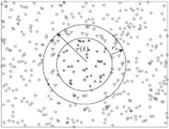
Fig.1. WSN Topology 1 [7,19]

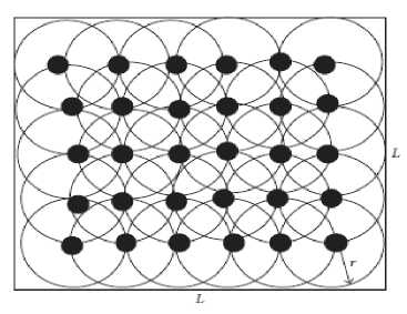
Fig.2. WSN Topology 2 [23]

• III.    The Seir-V Model With Vertical Transmission

Here, we propose the Vulnerable–Latent–Breaking Out–Temporarily Immune–Vulnerable with an Inoculation compartment ( VLBTV-I ) epidemic model. Specifically, we apply the Tang and Mark[7]’s and Feng et al. [23]’s expression for uniform random distribution of sensor nodes as well as Mishra and Pandey [11]’s expression for vertical transmission. Essentially, Vulnerable ( V ) sensors are susceptible to new infections and has no immunity, Latent ( L ) sensors are exposed to worm infection, Breaking out ( B ) sensors are infected and infectious, Temporarily immune ( T ) sensors have recovered from a worm infection and Inoculated ( I ) sensors are vaccinated against worm infection. The model investigates both horizontal and vertical worm transmission in a wireless sensor networks. Let V(t) , L(t) , B(t) , T(t) , I(t) denote the numbers of sensors at time t .

Li et al . assumed, “that a fraction of the offsprings of infected hosts (both L and B ) are infected at birth and, like adult infected hosts, will stay latent before becoming infectious, and hence the infected birth flux will enter the

L class”. Consequently, Mishra and Pandey [11] assumes that, “the birth flux into the exposed class is given by pbE + qbl and the birth flux into the susceptible class is given by b - pbE - qbl ”. This implies that a fraction p and a fraction q of the new nodes from the exposed and the infectious classes, respectively, are introduced into the exposed class. We adopt these assumptions too in the light of communication range and density; in our case herein the birth flux into the Latent (exposed) compartment is pAL + qAB and the birth flux into the Vulnerable compartment is Л- pAL - qA . Table 1 presents the meanings and names of several parameters employed for our WSN model formulation.

Table 1. WSN Parameters and Their Meaning

Parameters	Name	Meaning
p	p	Fraction of new nodes from the latent compartment
q	q	Fraction of new nodes from the breaking out compartment
X - pAL - qAB	-	Birth flux in the Vulnerable compartment
pAL + qAB	-	Birth flux in the Exposed compartment
A	lambda	Recruitment rate of vulnerable nodes to the sensor network
σ	sigma	Distribution density
	r	Transmission range
L2	-	Length of side
алгд	-	Effective contact with an infected node for transfer of infection (Topology 1)
алт02 / L2	-	Effective contact with an infected node for transfer of infection (Topology 2)
P	beta	Infectivity contact rate
	tau	Death rate of nodes due to hardware or software failure
to	omega	Crashing rate due to attack of malicious codes (in this case worm)
9	theta	Rate at which latent nodes enter the breaking out compartment
V	nu	Rate at which infected nodes become temporarily immune
Ф	phi	Rate at which temporarily immune nodes become vulnerable
p	rho	Rate of inoculation for vulnerable sensor nodes
	zeta	Rate of transmission from the inoculation compartment to the vulnerable compartment

Topology 1

Topology 2

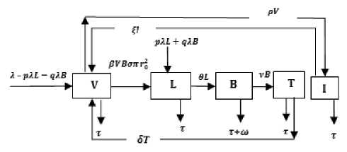
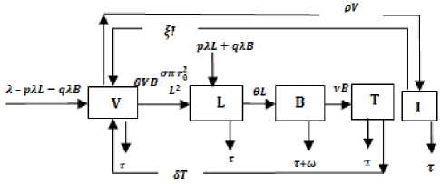
Fig.3. Schematic diagram of Topologies ((1) and (2)) for Wireless Sensor Networks

* _    (5+T)(v+ t+ _Ш)(Л— ^’^^^р^)¹¹ )

• ¹    St ( 0+v+ t) +5( 0+ t) 0+T)(v+т+to )

Сй+тчеел-Tf±P±lK(t-Pl±EK2TE+Lt£^₎ ’  ______________________ £С£+2222Цо___________

^L      8т ( 0+v + t) + 5( 0 + t) 0 + T)(v+t+to )

( f+P+T)(( в - p X +r)(v+ T +to)- q в X ) V ( 0 Л-- 5-------------- )

у ’ _ __________________ 3 ( f+ T) g TT r g ____________

^X     6 T(0+ v + T) + 6 (0 + t)(D + t( 0 + T)(v + T + to)

^о    p ((0—рЛ+ t)(v + t+to ) — q 0Л)

• ¹             P 0 (f+T) а П r^g

  
  

Topology 2:   Endemic equilibrium       =

(V ’ , L I .B ’ .T i’ .I i’ ) i.e.

The schematic diagram for the dynamical vertical and horizontal transmission of worms in a WSN given our assumption is depicted as Fig. 1. The system of differential equation (1) is adapted from Mishra and Keshri [4] but modified to capture distribution density, transmission range and vertical transmission.

The VLBTV-I Model 1 for topology 1 is represented using the following system of differential equations;

V = Л - PVBanr₀² - pAL - qBB - (т + p)V + TT + О

L = p VB anr₀² + pAL + qBB - (т + 6 )L

В = LL-(T + to+v)B            (1)

T = vB - (т + T)T i = p v - (T + oi

The VLBTV-I Model 2 for topology 2 is represented using the following system of differential equations;

V = Л - 1ТТ°Т_ - pAL - qBB - (т + p)V + TT + О

L = pVBaitr²/ L ² + pBL + qBB - (т + 6 )L

В = LL - (т + ^ + v)B             (2)

T = vB - (т + T)T i = pv - (т + 01

• A.    Solutions of Equilibrium Points

We equate the modified system of differential equations (1) to zero to obtain two solutions which are the Worm-free equilibrium and the Endemic equilibrium points i.e. V = 0; L = 0 ; B = 0 ; T = 0; / = 0 . The Worm-free equilibrium describes the absence of worms while the Endemic equilibrium describes the presence of worms in the Wireless Sensor Network using formulated mathematical model.

For both topologies (i.e. Model 1 and Model 2); the solutions       of       Worm-free       equilibrium

• ^V 0 = S o« = 0; ^B 0 = 0; ^t 0 = 0.« = ^ (3)

Topology 1:   Endemic equilibrium   E L  =

^о   ((0—рЛ+ t)(v + t+ to ) —q0Л)

1           ^вОПГд в 0

T 1 =

у о _ L²((0—рЛ+ t)(v+t+ та)— q 0Л)

1                 /?0СТТТГо

_     (5+T)(v+ t+ to)(Л—УТ^^+РТ^ТЕ))

• ¹    t ( 0+ t)(v + t +а)— S ( 0 ( t +to )+ t(v + t + to ))

0 (— ₅— t )(—v— t— а)(Л— V О ^^")¹⁷) )

(          )(   (         )    (     )      (     )(          ))

(L ² t( f+p + t) (— q 0 Л+( 0— p Л+ t) (v+ t +to ))— p 0 Л( f+т)о"тг r^g )

(     )(   (         )    (     )      (     )(          ))

r ’

(( 0— p Л+ t) (v+ t + to ) — q 6 Л) P 9 (f+ t) a nr²

• B.    Epidemic Threshold

The epidemic threshold can also be referred to as the Reproduction number denoted as R₀. The reproduction number is defined as “the expected number of secondary cases produced in a completely susceptible population, by a typical infective individual”[25]. Using the method that was used in Mishra and Pandey, [11], which regarded the Reproduction number as the inverse of the susceptible nodes (S j¹) at the endemic equilibrium; our Reproduction numbers here are;

Topology 1: R₀ = ------- ^ ^{00-71 r}°--------

((          )(         )       )

Topology 2: R₀ =  -----^°^²------

((          )(         )       )

In Mishra and Pandey [11], the reproduction number depends on the rate of the transmission from the exposed (latent) to the infectious (breaking out) class, the rate of the transmission from the infectious to the recovered class, the deaths as a result of the worm infections and other causes, the fraction of the exposed and infectious introduced into the exposed class. So is our reproduction number, but with the addition of the parameters for communication range and density. Note that the reproduction number of topology 2 involves L which denotes the length of side.

• C.    Stability of the Worm-free Equilibrium Point

We show the proof of local asymptotic stability at the Worm-free Equilibrium using the jacobian method. This is done by showing that “the eigen-values of the jacobian matrix all have negative real parts” [4] or that the “characteristic equation of the jacobian matrix” derived from the system of equations has negative roots [26].

Theorem 1: The worm-free equilibrium (for topology 1)

is locally asymptotically stable if RQ			< 1 and unstable if   The Jacobian matrix at				worm	free equilibrium point M^o
R0 > 1.				for topology 1 is;
/– рВаят 02- (T+			p )- pA	- рУаят 2 qA		5		f
		PBanr 02	–(T+ e )+	pA   /3Vanr 02+ qA		0		0
J =		0	e	–(T+w+V)		0		0		(6)
		0	0	V	–	(T+ 6 )		0
⎝		p	0	0		0	–	(T+)
		-(T+ p )	- pA	-     02A(f+ ) - QA (?+T)	5		f
	⎜	0–	(T+ e )+ pA	02A(f+ ) qA	0		0	⎞
J ( < ) =				( + )					⎟	(7)
		0	e	–(T+w+V)	0		0
		0	0	V          –(T+5)			0
	⎝		0	0	0		–(T+	)⎠

Theorem 2: The worm-free equilibrium (for topology 1)

is locally asymptotically stable if RQ < 1 and unstable if

RQ > 1. The Jacobian matrix at worm free equilibrium point И70 for topology 2 is

J = ⎜	– f^Banr 02 -(т+ P ) ⎛      P В аят 02 0		- pA –( T + e )+ pA e 0 0	- рУаят 02 / L - /3Vanr 02/ L 2+ i –( T +w+V) V 0	qA M	6 0 0 –(T+5) 0		f 0 0 0 –(T+
										f)⎠	⎟                   (8)
	⎝	0 P
		-(т+ P )	- pA       ■	-     02A(f+ ) L 2 (0 ?+;)     - qA	6		f
J (<) = ⎜⎜		0 0       –	( T + e )+ pA e	02^( 5 + )       , L 20( f+;)    + qA –( T +w+V)	0 0		0 0		⎟⎟		(9)
		⎝0	0 0	V                ■ 0	–( T + 0	6 ) –	0 (т+	f)⎠

Eigenvalues of (7) and (9) for both topologies are: -(T+ p ),–(T+ 9 )+ pA ,–(т+w+V), –(T+5), –(T+f) which all are negative; hence the system is locally asymptotically stable at worm free equilibrium point W₍f .

• IV.    Numerical Results and Discussion

The systems of differential equation ((1) and (2)) was solved using a numerical method i.e. Runge-Kutta Fehlberg method of order 4 and 5. This numerical method was used because it has been found suitable for a wide variety of initial value problems in practical applications. Subsequently we performed simulation experiments using the following initial values for the Wireless Sensor network: V=100; L=3; B=1; T=0; I=0. For the simulation experiments, we performed model alignment i.e. our model was docked to match (and compare our results with) the WSN model results in [4] and [27]. Summarily, Vulnerable, Latent, Breaking out, Temporarily immune, Inoculated in our model imply Susceptible, Exposed, Infectious, Recovered and Vaccinated respectively in [4,27]. Other simulation values include sigma=0.3; r=1;

lambda=1.2; tau=0.2; beta=1.3; phi=0.8; theta=0.4; nu=0.6; omega=0.3; delta=0.8; p=0.1; q=0.1; rho=0.1; xi = 0.1; adapted and modified from [11].

A. Numerical Simulation Results for Topology 1

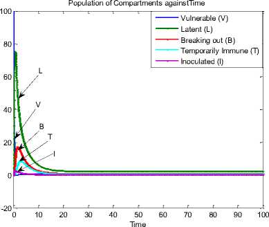
Fig.4. Sensor Population against Time at p= q=0.1

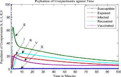
Fig.5. Sensor Population against Time [16]

(which is the recruitment rate of susceptible nodes to the sensor network) was kept constant at 1.2, all through the simulation in Fig. 7. Additionally, the infectivity contact rate or the effective contact rate (which results in horizontal worm transmission) was kept constant was also constant throughout the simulation in Fig. 7.

In Fig. 8 we kept p and q constant so as to elicit the actual effect of new sensor nodes added to the sensor network. This is because the relation (i.e. pAL + qAB ) that represents vertical worm transmission involves sensor node inclusion into the network. The inoculated (I) compartment in our model decreased greatly; however, Fig. 9 was plotted in a three dimensional form to show the effects of vertical worm transmission on the breaking out and the inoculated nodes.

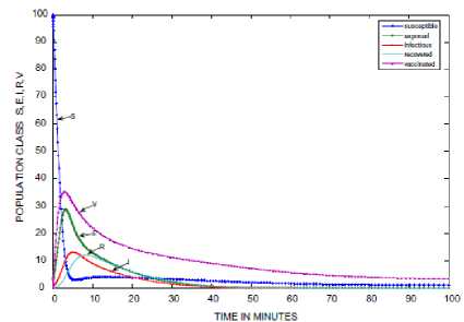
Fig.6. Sensor Population against Time [12]

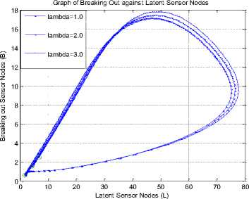
Fig.8. Breaking out vs Latent at p=0.1 and q=0.1

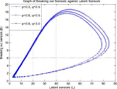
Fig7. Breaking out vs Latent at A = 1.2

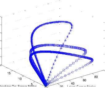
3 D Graph of Latent, Breaking out and Inoculated Sensor Nodes

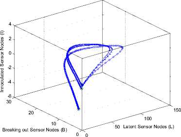
Fig.9. 3D Phase Plane showing L , B and I sensor nodes

Fig. 4, Fig. 5 and Fig. 6 are the time histories for our model herein and the WSN models in [27] and [4], respectively. A cursory look at the figures shows several differences. They include the almost disappearance of vulnerable nodes in our model. Then, the increase in the number of latent (exposed) sensor nodes in our model compared to responses from other models. Note that the increase in density and range increased the exposed nodes in both our study and in [27]; since the model in [4] doesn’t entirely depict a wireless sensor network.

Keeping p constant (at 0.8) and keeping q constant (at 0.5) depicts the effect of vertical worm transmission in Fig. 7. This figure shows that increasing the fraction of latent nodes ( p ) and the fraction of breaking out nodes ( q ) introduced into the breaking out compartment ( B ) increased both B and latent ( L ) compartments. Note that A

Graph of the Impact of Recovery and Vaccination

Latent Sensor Nodes (L)

Fig.10. Breaking out vs Latent Sensor Nodes

Fig. 10 depicts the impact of increasing both the rate at which nodes become temporarily immune to worm infection and the rate of inoculation. From the diagram, it is evident that the rate of infectiveness (or break out) for both the latent/breaking out sensor nodes reduced to 62/7 from a high value of 75/18. Correspondingly, the rate of sensor inoculation was increased (in Fig. 11) from below 10 to almost 40 as a result.

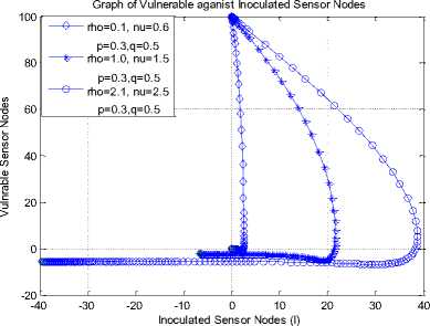
Fig.11. Vulnerable vs Inoculated Sensor Nodes

Graph of the Impact of Horizontal Transmission through Effective Conatc 20

0     10    20    30    40    50    60    70    80    90    100

Latent Sensor Nodes (L)

Fig.12. Breaking out vs Latent Sensor Nodes

3D Graph of Latent, Breaking out and Inoculated Sensor Nodes

CO

2.5

1.5

0.5

Breaking Out Sensor Nodes

20 Latent Sensor Nodes

Fig.13. 3D Phase Plane showing L, B and I Sensor Nodes

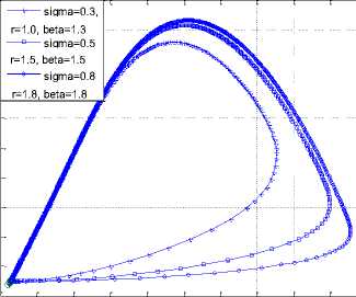
Fig. 12 and Fig. 13 were used to depict the impact of horizontal transmission (by increasing the parameters that form the effective contact rate i.e. апгц ) in Model 1.

While Fig. 12 shows the relationship between latent and the breaking out sensor nodes using a two dimensional graph, Fig. 13 shows the relationship between latent, breaking out and the inoculated sensor nodes using a three dimensional phase plane. Summarily, the two plots showed how horizontal worm transmission in Model 1 increases infectiousness.

• B.    Numerical Simulation Results for Topology 2

The two proposed models herein are mostly the same, if not for the addition of length of side ( L² ) in the topological expression in [23]. There is the implicit (and accurate) assumption that the above simulation results of Model 1 would be “ almost” the same with the results of Model 2, if simulated with the same values. Therefore, we perform simulation experiments in order to elicit the impact/effect of the length of side, existent in Model 2.

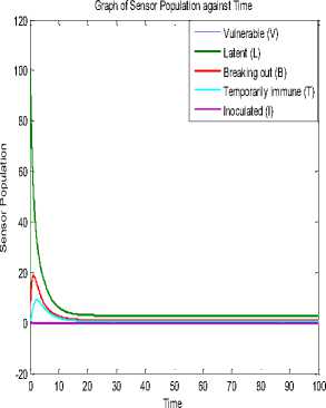
Fig.14. Sensor Population against Time at L =0.1

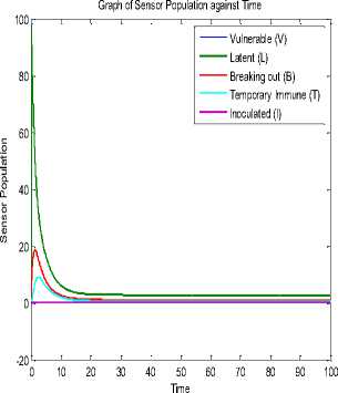
Fig.15. Sensor Population against Time at L =0.2

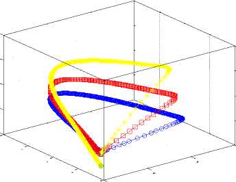
Fig. 4 and Fig. 14 are almost the same; only that the inoculated nodes became zero and the vulnerable nodes disappeared in the latter; so is Fig. 15. The three figures were simulated with the same values except for the addition of L2=0.1 in Fig. 14 and L2=0.2 in Fig. 15. Fig. 16 depicts a three dimensional plot of the dynamical relationship/behavior of latent, breaking out and inoculated sensor nodes. It also shows the corresponding decrease in the inoculated nodes. The effect of the length of side (L2 ) is clear if one compares the 3D phase plane of Model 1 (Fig. 13) and that of Model 2 (Fig. 16). Recall that L2 is part of the parameters that constitute the effective contact rate in Table 1. The effect of increasing the factors of vertical transmission and L2 is evident if one compares Fig. 16 and Fig. 17.

3D Graph of Latent, Breaking Out and Inoculated Sensor Nodes

0.5

0.4

0.3

0.2

0.1

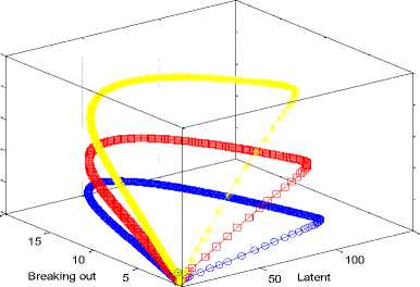
Fig.16. 3D Phase Plane showing L, B and I sensor nodes at L² =0.1, 0.2, 0.3; p=0.1 and q=0.1

3D Graph for Latent, Breaking out and Inoculated Sensor Nodes

0.6

0.4

0.2

-0.2

10 Breaking out

50 Latent

Fig.17. 3D Phase Plane showing L, B and I sensor nodes at L² =0.1, 0.2, 0.3; p =0.3, 0.8, 0.8 and q =0.5, 0.5, 3.5

• C.    Analysis Using the Epidemic Threshold

Here, we present the actual values for the epidemic threshold (reproduction ratios) derived at Section III using the time histories of Model 1 (Fig. 4), Model in [27] (Fig. 5), Model in [4] (Fig. 6) and Model 2 (Fig. 15). Table 2 presents the reproduction numbers for the time histories of the study herein. This would further display the impact of vertical worm transmissions in the wireless sensor network.

Going by the fact that at Rq < 1 the infection is contained and at Rq ≥ 1 the infection spreads and there is an epidemic; Table 2 displays interesting results. Note that the rationale for comparing our study herein and the models in [4] and [27] is because they all involved the SEIR-V epidemic model. Table 2 shows that Fig. 6 of [4] has the lowest reproduction number; this is because it is unlike Fig. 4 and Fig. 15

that involved range, density and vertical transmission. The impact of characterizing range and density without vertical transmission is expressly shown in the difference between Fig. 4 and Fig. 5 or the difference between Fig. 5 and Fig. 15. The table also shows that vertical transmission for both topologies made Rq to rise above 1. Furthermore, the reproduction number for topology 2 i.e. Fig. 15 significantly rose beyond 1 to 25.529. To prevent epidemic, network managers should strive to keep the reproduction numbers below 1.

Table 2. Time Histories and their Reproduction Numbers

Figures	Parameters Considered	Reproduction numbers
Fig. 4.	Vertical       transmission, Range    and    Density (topology 1)	1.021
Fig. 5. [27]	Range    and    Density (topology 1)	0.788
Fig. 6. [4]	---	0.209
Fig. 15.	Vertical       transmission, Range    and    Density (topology 2)	25.529

• V. Conclusion and Future Directions

In this study, we characterized and investigated both vertical and horizontal transmission of worms using two epidemic WSN models. These two epidemic models represented the topological expressions for uniform random sensor distribution, and are culled from [7, 19] and [23]. Vertical and horizontal worm transmissions are studied alongside these expressions. Thereafter, a suitable numerical method for an initial value problem was chosen to solve, simulate and validate these proposed models.

WSN characterization using two topologies culled from literature was necessary because it aided the derivation of novel reproduction numbers. Note that the WSN models that underpin this study presented reproduction numbers that characterize only horizontal worm transmission. However, the reproduction numbers (of our study), which differ from (those in) underpinning works depicts the resulting secondary infections when vertical transmission, communication range and distribution density are put into consideration.

Vertical worm transmissions increased the latent and the breaking out sensor nodes by the introduction of new births, so was horizontal worm transmissions. However, the negative impact of these worm transmissions was significantly reduced by increasing correspondingly the rate of temporary immunity and the rate of sensor inoculation. Noteworthy is the fact that temporary immunity achieved by increasing V (nu) quickly becomes of no effect due to the existence of another worm variant or another malicious code type.

In furtherance, we would check the effect of vertical transmission on other network countermeasures such as quarantine, network access control etc. Additionally, we would explore the possibilities of using a different modeling approach such as agent modeling (ABM) in order to represent and analyze the import of other instances of stochasticity and heterogeneity in wireless sensor networks.

Acknowledgment

We thank the anonymous reviewers that read our manuscript and their keen efforts directed at ensuring accuracy of our work.