Towards monitored tomographic reconstruction: algorithm-dependence and convergence

X-ray computed tomography is widely used in medicine [1 –5], industry [6, 7], customs control [8] and in research [9– 11] as a non-destructive method for visualizing the internal morphology of objects. Tomographic measurements are performed on various scales, up to nanometer spatial resolution [12]. Each specific application imposes its own limitations on the method. Thus, medical applications require to limit the radiation dose load on the patient, while in industrial application the inspection time is critical. A reduced time-to-data is essential for laboratory nano-XCT studies, which usually take hours. Both goals of radiation dose and measurement time reduction can be achieved by reducing the total number of X-ray projections (views). However, the number of projections and the quality of the reconstruction, including spatial resolution, are tightly related to each other [13]. Reducing the number of projections inevitably leads to a loss of reconstruction quality. At the same time the behavior of image degradation with reduction of projection count may depend on various factors, such as choice of the reconstruction algorithm [14], scanning scheme type, size of the region under reconstruction, required spatial resolution [15]. While a lot of efforts to reduce the number of projection have been made, simultaneously, new algorithms are being developed to perform reconstruction with fewer projections [16– 18]. However, it is not easy to develop and approve the tomography data collection protocol to comply with an “as low as reasonably achievable” requirement to the total dose, since one has to predict the exact number of angles required to obtain an image of such quality as it is necessary for a diagnostic conclusion or for defect inspection.

Recently, a new approach to the tomographic process, called monitored tomographic reconstruction (MTR), was suggested [19]. The ordinary tomographic study can be seen as a two-stage process, which includes the data collection and the image reconstruction, which is performed only after the full dataset has been acquired. It was suggested to replace the classical process with an any-time process [19–21], in which the acquisition of projections is interspersed with image reconstruction. The automatic stopping of the scanning process for the currently scanned object occurs according to a certain rule. The theoretical background for the stopping rule construction and the theoretical framework for the monitored reconstruction was given in [19]. In this paper, for the first time, we systematically apply the MTR technique to numerical data from experiments performed using XCT technique wiht differences in photon energy ranges, geometries as well as fild-of-view and resolution. The following reconstruction algorithms were included into the MTR protocol within the conducted experiments: Filtered Back Projection (FBP) [22], Hough based Filtered Back Projection (HFBP) [23], Direct Fourier Reconstruction method [24], Simultaneous Iterative Reconstruction Technique (SIRT) with Total Variation (TV) regularizetion [25] and Hough-based Simultaneous Iterative Reconstruction Technique with Total Variation (HSIRT-TV) [26]. To estimate the current reconstruction error in MTR experiments, we used two types of ground truth images. The first one is the image reconstructed with the same reconstruction algorithm as used in the MTR experiment with a full set of projections. We call it an algorithm- dependent ground truth. Its usage is justified by the fact that the MTR protocol influences the number of projections used for each given object, thus effectively only influencing the reconstruction artifacts due to absence of a full set of projections. The second ground truth image is the reconstruction result obtained with SIRT-TV, where the FBP reconstruction result is used as the initial approximation for the SIRT iterative procedure with an extensive number of iterations. We call it independent ground truth. Both ground truth images are calculated with a full set of projections collected during the XCT measurements. The tomography dataset used for the MTR properties study was collected from two different laboratory XCT setups, nano-XCT and micro-XCT. The first one has X-ray optics installed in the beam path, which makes it possible to carry out the measurements with a resolution of several 10 nm. In this particular example, the field of view is 65×65 microns, and the lateral resolution is about 65 nm [27]. The field of view of the second tomography setup is about 1×1 cm, and the spatial resolution is 10 microns [28].

The following parts of the paper are organized as follows. Section “Materials and Methods” contains a description of the nano-XCT and micro- XCT setups, the description of the measured samples, description of Smart Tomo Engine tomography reconstruction tool used in MTR experiments, and framework of MTR experiment. The next section presents a description of MTR experiments in detail. The last section presents the discussion of the obtained results.

1.    Materials and Methods 1.1.    Nano-XCT laboratory setup

The acquisition of the nano-XCT data was performed using an Xradia nano-XCT 100 setup (Xradia Inc., Pleasanton, CA, USA). The laboratory nano-XCT setup consists of the following main components: an X-ray source with a rotating anode e mitting CuKa radiation (8 keV photon energy), an illumination system consisting of a capillary condenser optics with a central beam stop, a Fresnel zone plate (FZP) as an objective lens enabling sub-100 nm resolution and a scintillation detector including a CCD camera (1024×1024 pixels). Such setup provides nearly parallel-beam imaging, and it allows to obtain X-ray computed tomography data within an angular range of 180 ° , compared to usually 360 ° . The scheme of the X-ray microscope beam path is presented in Fig. 1.

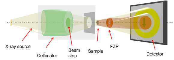
Fig. 1. Optical beam path of nearly parallel-beam geometry for a nano-XCT setup

• 1.2.    Description of nanostructures on the study

The sample studied consists of needle-like MoO2 micro-cuboids as parts of a novel, hierarchically structured transition-metal-based electrocatalytic system with high electrocatalytic efficiency for hydrogen evolution reaction (HER): MoNi4 /MoO2 @ Ni) [29]. The MoO2 micro cuboids that have a rectangular cross-section of 0.5×1 µm2 and a length of 10 to 20 µm were detached from the nickel foam and fixed on a tiny needle acting as sample holder [12]. High-resolution XCT provides 3D information of the hierarchi- cal morphology of the MoNi4 /MoO2 @Ni material system and particularly of the arrangement of the MoO2 cuboids nondestructively. The X-ray com- puted tomography scan was performed in standard resolution mode (40 FZP magnification 20 optical magnification = 800 total magnification). The width and height of the field of view (FOV) were 65 µm with 1024 pixels for each, resulting in a pixel size of 65×65 nm2. The X-ray computed tomography data were collected in the 180° angular range, and they included 801 images which were acquired with an exposure of 180s each.

• 1.3.    Micro-XCT laboratory setup

  X-ray computed tomography measurements were performed on a “TOMAS” laboratory micro-XCT setup Fig. 2 developed and constructed in FSRC “Crystallography and Photonics” RAS [28]. The X-ray tube with a molybdenum anode (emitting Moka photons with a characteristic energy of 17 . 5 keV ) at the accelerating voltage 40 kV and anode current 20 mA was used as a radiation source. The measurements were performed using a pyrolytic graphite crystal as a monochromator. The monochromator-sample distance was 1 . 2 m, and the sample-detector distance was 0 . 02 m. The size of the X-ray beam on the object position was about 2 cm. In each experiment, 400 projections were taken in the angular range of 0200 ° , in 0 . 5 ° increments and 5 seconds per frame exposure. A XIMEA xiRay 11 high-resolution X-ray detector with 9 µm spatial resolution and at a field of view of 36×24 mm was used in the measurements.

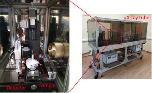
Fig. 2. Picture of the laboratory micro-XCT setup with nearly parallel-beam geometry and monochromatic X-ray radiation

• 1.4.    Description of objects on the study with micro-XCT

For testing the MTR technique, we collect a dataset of the objects with different morphology (biological samples, plastic, and calcium). Here is a description of the samples on the study:

• •    The top part of the toothbrush (Fig. 3 а ) is a rubber and plastic sample, contains many plastic fibers, and has many contrast edges.

• •    The shell (Fig. 3 b ) is a simple hollow sample consisting mainly of calcium oxalate.

• •    The larch cone (Fig. 3 c ) is an organic object with complex geometry.

• •    The raspberry fixed on a plastic base (Fig. 3 d ) is an organic sample containing a lot of liquid. Sample fixed on the plastic tube to keep the form during measurements.

• •    The apple seed (Fig. 3 e ) is a small organic sample with a relatively homogeneous structure.

• 1.5.    Smart Tomo Engine tomography reconstruction tool

The Smart Tomo Engine (STE) is a tomography data processing, reconstruction and visualization software solution developed by Smart Engines Service LLC [30].

STE is a cross-platform software that implements fast and precise reconstruction algorithms, artifacts reduction methods and data 2D and 3D visualization. The typical STE tomography reconstruction workflow consists of the following steps: loading the source data, correcting geometry parameters (like rotation axis position search and correction), tomography reconstruction, artifacts reduction and visualization. The input set of projections can be loaded from different types of format – TIFF (float32, uint16, uint32), PNG (uint16, uint32), DICOM [31], DICOMDIR, Nexus [32]. At the first stage of loaded data processing, the flat field correction is performed: the dark current is taken in to account if such frames are present in the in- put dataset; then the images are normalized to frames of the empty beam and, if necessary, the logarithm is taken. Additionally, the STE can automatically search for the axis of object rotation, perform correction of ring artifacts and automatically correct data in order to suppress artifacts caused by polychromatic radiation.

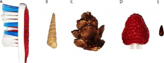
Fig. 3. Picture of objects in micro-CT dataset: A – toothbrush, B – shell, C – larch cone, D – raspberry, E – apple seed

Reconstruction algorithms for layer-by-layer 2D and/or true 3D reconstruction of received data with a circular scan path are also available in the Smart Tomo Engine. In STE we use classical reconstruction algorithms, such as Filtered Back Projection (FBP) [22], Feldkamp, Davis and Kres algorithm (FDK) [33], Direct Fourier Reconstruction method (DFR) [24], Simultaneous Iterative Reconstruction Technique (SIRT) with Total Variation (TV) regularization [25], the fastest and the most modern algorithm reconstruction algorithm - Hough based Filtered Back Projection (HFBP) [23] and the fastest iterative reconstruction algorithm – Hough based Simultaneous Iterative Reconstruction Technique (HSIRT) [26]. STE implements x64 compatible CPU, ARM processors, and GPU accelerators (CUDA).

The result of the reconstruction can be viewed layer by layer, in different color palettes or in a 3D visualizer. The 3D visualizer presents three types of visualization of the reconstructed volume: monochrome, translucent color and solid visualization. A monochrome rendering type is a grayscale rendering of an image. Type translucent color displays a three-dimensional reconstruction in the form of a translucent volume, according to the laws of light absorption. The solid type renders a 3D continuous iso surface, while the brightness level is set by the user himself in the graphical interface. The reconstruction result can be saved layer by layer in TIFF, PNG, DICOM formats, as well as in a two-dimensional image of threedimensional visualization.

The result of the 3D reconstruction from the set of projections for all objects is presented in Fig. 4. A Filtered Back Projection algorithm was used for reconstruction to produce illustrations.

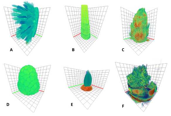
Fig. 4. Reconstructed volumes from all collected projections. Objects for Micro-XCT setup: A – toothbrush, B – shell, C – larch cone, D – raspberry, E – apple seed. Object for Nano-XCT setup: F – needle-like MoO 2

• 1.6.    Description of used tomographic reconstruction algorithms

For our experiments, we choose four different reconstruction algorithms, each having an implementation in STE, namely: commonly used Filtered

Back Projection (FBP) [22], Hough based Filtered Back Projection (HFBP) [23], Direct Fourier Reconstruction method (DFR) [24], Simultaneous Iterative Reconstruction Technique (SIRT) with Total Variation (TV) regularization [25] and Hough based Simultaneous Iterative Reconstruction Technique (HSIRT) [26]. Since all the data is acquired in parallel geometry, all of the further discussed implementations are also meant in terms of the parallel geometry of the experiment. Also, reconstructions of a single layer as a 2 D image are discussed, and all the complexity should be understood in terms of reconstructing a single layer and not an entire volume. The complexity of the algorithms given below is calculated in the assumption that detector size n reconstructed image width number of projections number of reconstructed layers.

Here we want to explain the choice of these algorithms together with their key features. FBP algorithm implements Fourier filtration of obtained projections by the Ramp filter with the following backprojection of filtered data. The FBP algorithm offers a good tradeoff between speed ( O ( n ⁴ ) complexity) and quality of reconstruction, which makes it an algorithm of choice for a wide range of tomographic tasks. FBP also provides a good baseline for comparing different algorithms. The HFBP algorithm utilizes the Transposed Fast Hough transform of an image to significantly speed up the Back Projection part of FBP, resulting in

O ( n ³ log ( n )) complexity. It should be noted that in HFBP all the lines are approximated by pixel patterns on an image, which usually results in slightly worse quality of an image in comparison with HFBP. However, the high speed of this algorithm makes it quite a good candidate for use during the monitoring reconstruction process. DFR algorithm is making use of Fourier slice theorem [34] by creating a full 2D Fourier image from filtered data with the following 2D Inverse Fourier Transform to produce reconstruction. The image quality of the DFR method com- pared to FBP usually suffers from an irregular sampling of points in Fourier space. Although DFR is another algorithm with O ( n ³ log ( n )) complexity which makes it worth studying its properties in the framework of monitored reconstruction. Algebraic algorithms such as SIRT or HSIRT aim to minimize the reprojection error by performing an iterative search. Each iteration of such an algorithm requires 2 to 3 operations of forward and backward projections, which makes if 2× k times (where k is the number of SIRT iterations) slower than the corresponding Filtered Back Projection algorithm and makes it impractical to use such algorithms in monitoring reconstruction. Although algebraic algorithms such as SIRT and HSIRT provide relatively fast convergence in terms of projections count, which may (or may not) be an important property considering monitoring reconstruction protocol and the other considered algorithms do not possess such a property.

• 1.7.    Monitored reconstruction

2.    Description of numerical experiments 3. Results and discussion

The MTR technique relies on analyzing intermediate reconstructions of an object during CT measurement to achieve dose reduction for a predetermined reconstruction quality. The detailed description of the framework may be found elsewhere [19, 27], here we will only briefly discuss the most general aspects of this approach and the details specific for the present experiments. The task for MTR is formulating as minimizing the loss function in the space of number of acquired projections. Loss function L may be written in form L = E (err ( N )) +cost ( N ). Here E (err ( N )) is an expected value of an error calculated by some chosen metric between reconstruction from N projections and ground truth image; cost ( N ) is the cost function of acquiring N projections, which is usually chosen to be a linear function cN , where c is the cost of obtaining one projection. Solving this optimization task is significantly complicated by the fact that the error should be calculated relative to an ideal reconstruction which in practice will not be available during the MTR process. This means value E (err ( N )) should be calculated only on the base of preceding history of partial reconstructions. In the fair assumption of derivative of E (err ( N ) being monotonous by N and considering two neighboring points i and i + 1 the stopping rule may be formulated as err ( N i ) E (err ( N i +1 )) <  c .

In the framework we chose a simple approach for calculating d (err ( N ))/ dN function estimating it as the ℓ 2

norm of a difference between two neighboured partial reconstructions. To compare the effectiveness of the stopping rule one can calculate different metrics, even the ones calculated from ideal reconstructions or reconstructions from full projection data.

solution for 150 iterations of SIRT with TV regularization.

This way the results of our experiments are going to be an average error plots for naive and monitoring rules each for a fixed algorithm, dataset and GT images set.

Most numerical experiments were reproduced following the paper [27].

The experiments consist of 4 main stages:

• 1.    Preparing dataset and ground truth images.

• 2.    Choosing a reconstruction algorithm and collecting partial reconstruction data.

• 3.    Estimating baseline average error across all the objects for every stopping point.

0.60 0.60

Estimating average error across all the objects for each threshold value using the monitoring rule.

Further, we should consider these stages more closely. Two real data datasets were prepared. The first dataset was created from different slices of a single object, collected on nano-XCT setup (NanoCT dataset), the second dataset was created from from different objects, collected on micro-XCT setup (MicroCT dataset). The monitoring rules cannot have any knowledge about target ground truth (GT) in the process of acquisition, although to conveniently plot the error for all the algorithms, we would still need GT images. Following the paper [19] we reproduce the experiments using as GT the last, full-dose image. We will also compare different algorithms against a common GT to validate the convergence of algorithms. The common GT images are constructed from full projection data using the FBP algorithm as the initial

The main result of the experiments described in the previous part is an average reconstruction error corresponding to a different mean number of projections. Although it is convenient to start the discussion by considering the derivative data which is responsible for choosing a stopping point for each of the different objects in the dataset. On Fig. 5 ℓ 2 norm of the difference between two consecutive reconstructions is represented. Any horizontal line on these plots would correspond to a fixed threshold c , and the first intersection of such a line with a plot would correspond to a stopping point for a particular object. It is worth noting that the general behavior for all of the algorithm /object pairs is common and may be described as a monotonous decay. The behavior of the integral algorithms (FBP, HFBP, DFR) is similar between themselves even quantitatively, although the algebraic algorithms (SIRT, HSIRT) differ quite a bit, which is most likely due to a better stability of these methods at smaller projections count. From Fig. 5 one can deduct that at a fixed c value all algorithms would in fact stop at different numbers of projections for different objects. While this is an essential and required property for monitored reconstruction to be able to demonstrate dose savings in comparison to a trivial stopping rule, this alone is not enough to guarantee that.

a) FBP

b)HFBP

0.60

C) DFR

0.50

0.50

0.50

8 0.40 s

5 °'30

5 0.20

8 0.40

I 0.30

5 0.20

У 0.40

5 0 30

5 0.20

0.10

0.10

0.10

0.00 40

0.60

Number of acquired projections

________________ d) HSIRT50

0.0010

200 Number

400      600

of acquired projections

0.60

0.001 0

200      400      600

Number of acquired projections e) SIRT50

0.50

8 0.40 $

5 0:30

5 0.20

0.10

0.0010

100    200    300    400    500    600    700    800

Number of acquired projections

0.50

У 0.40

£ 0 30

5 0.20

0.10

0.00 40

100    200    300    400    500    600    700    800

Number of acquired projections

Fig. 5. ℓ 2 norm of the difference between two consecutive reconstructions for all of the investigated algorithms

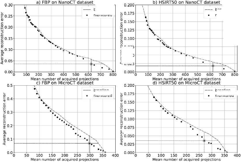
To find out if there is a possibility to achieve a dose reduction while producing a predetermined average quality we need to estimate these values for all possible thresholds c. Considering the GT to be a full dose reconstructions with the same algorithm, mean quality can be plotted against mean projection count in a way similar to [19] (Fig. 6), exampled graphs represent the results of MTR implemented on FBP and HSIRT algorithms on NanoCT and MicroCT datasets. In the high projection count region these plots demonstrate significant gain by both average dose and quality of monitored rule over the baseline (where non-monitored baseline is the stopping by the fixed number of projections). To estimate the maximum gain a close to optimal values of c are chosen for each individual graph. These points are circled on the plots on Fig. 6, and the gain here can be estimated as the difference between optimal point and baseline by either average projection count or reconstruction quality. Similar procedure was conducted for for all algorithms on both datasets and the results are brought together in Table 1. Since the dose is proportional to the projection count an average dose reduction may be calculated as the relation of difference in projection count to a total projection number. These results may be understood as in average a lower projection count is needed for the same quality across investigated objects or the better quality may be achieved for the same projection count. The values of dose reduction under the condition of the same average quality are only slightly varies in case of NanoCT dataset (5.0 – 10.0 %) and in case of MicroCT dataset (11.2 – 12.5 %). Since such payoff is achieved for all studied reconstruction algorithms, general stability of MTR protocol may be concluded.

baseline monitored

monitorec

? 0.050

Fig. 6. An example of average error (ℓ 2 norm of a difference from recon- struction by the same algorithm at full projection data) and mean number of projections for four of the investigated algorithms on NanoCT dataset. Dash lines represent trivial stopping rules (by the fixed number of projections), dots represent monitored stopping rules. A circled points represent close to optimal stopping points with an expected gain over baseline rule

c 0.075

2 0.050

< 0.025

baseline

baseline

monitored

baseline

monitored

Tab. 1. The gain in dose and quality achieved by MTR over baseline protocol

Algorithm	NanoCT dataset		MicroCT dataset
	Quality	Dose, %	Quality	Dose, %
FBP	0.05	8.75	0.02	11.2
HFBP	0.045	8.75	0.017	12.5
DFR	0.030	5.0	0.018	12.5
HSIRT50	0.030	10.0	0.011	12.5
SIRT50	0.030	10.0	0.011	12.5

We also aim to study the convergence of algorithms to an independent GT images described in previous section. Using a common GT for different reconstruction algorithms allows to plot the results of application of the MTR rules in a single scale (Fig. 7). The plots demonstrate that the algorithms reasonably converge to the common GT images although the gain in this case is much less significant. It is also should be noted that two different regions exist on the plots, nominally divided by the vertical dash line. Left region here correspond to undesirable image quality, and the stopping in this region is undesired under optimal conditions, even if there would be a gain in image quality or dose. The right region corresponds to a meaningful part of the curve, where some stopping point is expected. The difference between these regions is also illustrated on Fig. 8, where a partial reconstructions by FBP algorithm are represented for example objects from both datasets. Fig. 8 (b) and (e) demonstrate a borderline image quality below which an MTR algorithm should not be calibrated to stop in real experiments.

It should be noted that in all experiments each algorithm is compared against its own baseline, due to the chosen framework in which the same algorithm is applied for estimating the stopping point and for evaluating the final error. This shouldn’t be the case for the practical applications since after the data was acquired one does not have time restrictions and is free to use algorithms providing the best quality. Although from a theoretical point of view the algorithm used for monitoring reconstruction is aimed to minimize its own average error and in general does not guarantee that an average error/projection count for another reconstruction algorithm would also decrease.

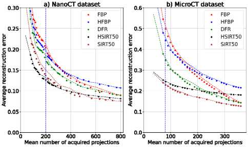
Fig. 7. Average error (ℓ 2 norm of a difference from common GT images) and mean number of projections for all of the investigated algorithms on NanoCT dataset and (b) MicroCT dataset. Dash lines represent trivial stopping rules (by the fixed number of projections), dotted curves represent monitored stopping rules

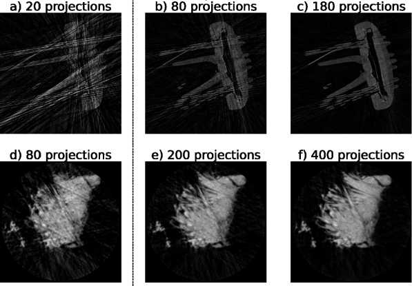
Fig. 8. Example partial reconstructions of objects taken from MicroCT dataset (upper row) and NanoCT dataset (lower row). Figures (b) and (e) corresponds to a vertical dash lines positions on Fig. 7

Conclusions

In this paper we conducted a series of studies of the effect of monitored tomographic reconstruction (MTR) with respect to different XCT setups, reconstruction algorithms, and approaches for quality estimation. It was shown that the reduction of the mean number of projections with retaining of the mean quality when stopping the reconstruction process according to the MTR protocol happens in every setup and reconstruction algorithm combination. The conducted experiments demonstrate that dose reduction properties are sustained between the different reconstruction algorithms included into MTR framework, while the algorithms still reasonably converge to the common GT reconstruction.

We were able to reproduce the result of [19] and generalize it to the case of different reconstruction algorithms included within the MTR protocol. The results represented in Table 1 demonstrate the significant gain in dose reduction for all algorithms on both datasets, and the dose reduction values reaches 12.5 % on MicroCT dataset and 10.0% on NanoCT dataset.

Although several implementation tasks have to be performed for the MTR implementation to a real hardware setup being connected with “calibration” procedure of the MTR protocol, the approach as described id formulated. During a “calibration” procedure a threshold c should be set in advance for an expectation of the reconstruction quality, which should then be converted to a stopping threshold. This stopping threshold in general is not guaranteed to be transferable between protocols (whether between setups or between re- construction algorithms), and as evident from the performed evaluation, the “calibration” will have to be based on the same reconstruction method as the one used during the scan. We rely on the existing methods of reconstruction and image quality estimation, common for the CT field, although these methods are limited in terms of applying to partial data. The reconstruction time emerges as a particular critical issue for this task, due to the real time nature of the protocol. Even though the technique MTR already demonstrates a success in dose reduction and acquisition time reduction, the research and development of new reconstruction approaches both fast and adequate to MTR tasks would be necessary to utilize these results in real XCT setups.