Towards Performance Evaluation of Cognitive Radio Network in Realistic Environment

Published Online November 2013 in MECS DOI: 10.5815/ijcnis.2014.01.09

Cognitive Radio Network (CRN) [2-3] is the current wireless technology requirement as it solves the problem of spectrum scarcity. CRN employs two categories of nodes [2-5]: Primary User (PU) and Secondary User (SU). The PU is allocated a license spectrum and can use it whenever it wishes to do so. The SU communicate through the licensed spectrum of PU nodes whenever the channel is not occupied by the PU node i.e. in CR technology the licensed spectrum of existing wireless network is utilized opportunistically. Whenever the PU’s become active the SU nodes must give up the communication channel for use by PU and switch to another channel if available. Various researchers have developed routing strategies that have proved beneficial in utilizing spectrum efficiently [16-18]. To evaluate the efficacy of these routing protocols simulation tools such as QualNet, NS2 and Glomosim are used. The simulation tool [6-7] provides a platform with specific advantage over real world as follows:

• A.    Repeatable scenarios

The protocol developers require changes to the protocol and retest the protocol in the same scenario. Hence this feature aids in deeper understanding of how the changes impact the performance of protocol. To implement this feature in real world, significant work needs to be performed.

• B.    Isolation of parameters

The feature helps the protocol designers to find the impact of single parameter such as mobility; bandwidth and transmission range [5-8], while keeping the other parameters constant. This feature is quite difficult to implement in real world.

• C.    Variety of scenarios and network configurations

The feature helps the protocol designers to change the scenario properties such as: number of nodes can be altered or data link layer protocol can be changed. Implementing this feature in real world requires much more duration and labor.

All of these advantages are not available with real world experiments. Due to these benefits, simulation tool has become a popular tool for the development. An important component of the simulators is the simulation region in which the nodes are to be deployed. The simulation region may contain obstacles [8-9] of varying shape and may contain varying number of obstacle. Moreover the obstacle may be of different types for instance river and mountain type. The former type obstacle restricts node movement only where-as the latter one restricts node movement as well as effective transmission range of the nodes. In addition to above, another factor of simulator is the shape of the simulation region in which the nodes are to be deployed. All these factors significantly affect the performance of routing protocols. Therefore to make the study exhaustive following experiments are performed.

• D.    Experiment 1

Evaluating the Impact on network performance by considering obstacles of different shapes in the simulation region.

• E.    Experiment 2

Evaluating the Impact on network performance considering obstacles of different types in the simulation region.

• F.    Experiment 3

Evaluating the Impact on network performance by considering obstacles of different sizes within the simulation region.

• G.    Experiment 4

Evaluating the Impact on network performance by considering the obstacles and varying the shape of simulation region.

To perform these experiments a simulator was designed in MATLAB-7. The paper also discusses the reasons for the variations in results in realistic and idealistic environment. The rest of the paper is organized as follows: Section 2 Illustrates the Literature Survey. Section 3 gives Algorithm and simulation set up parameters. Section 4 provides the impact of realistic scenario on CRN. Section 5 present the conclusion followed by the references.

• II.    LITERATURE SURVEY

There are only few researchers who have tried to make simulation as realistic as possible. Their work is as follows.

The work done by Amit Jardosh et. al. [8] was the first in the direction of making the scenario realistic. They incorporated obstacle in the simulation region of ad hoc network and observed that the use of obstacle or realistic condition not only reduces packet delivery ratio but at the same time increases the end to end delay of data packets.

A different strategy was adopted by N Meghanathan [9] to make the scenario realistic. Their paper showed that the performance of the ad hoc network starts deteriorating as the skewed ness of periphery from square to rectangle increases i.e. as the length to breadth ratio increases the performance of ad hoc network falls significantly.

Further comprehensive study on the shape of the simulation area and type of the obstacle was carried out by C. K. Nagpal et. al [1]. According to their observation, not only the shape of the periphery but the type (mountain or river) and number of obstacle also influences the performance of routing protocols of ad hoc network.

All these mechanism have been developed for ad hoc network and none of the researcher has made an attempt to incorporate realistic conditions in CRN environment. Thus this paper is written by keeping the following objectives in mind.

• 1.    To make the scenario realistic by incorporating obstacles of different types and analyze the cause of the same on performance of CRN.

• 2.    To vary the shape of the periphery and analyze the cause of the same on performance of CRN.

• 3.    To show that realistic results are quite different from idealistic ones

• 4.    To vary the concentration as well as time allocated by PU’s to SU’s in realistic condition thus showing the need for CRN.

We are of the opinion that before deploying any protocol, the geographical shape and the obstacle shape as well as number of obstacle in the region should be incorporated in the simulation software so that a true picture can be obtained about the protocol which is best suited under the given environmental conditions. The next section discusses the experiments performed by us to study the effect of same on the efficacy of routing protocols.

• III.    SIMULATION AND ALGORITHM

• A.    Performance Metrics

The following metrics has been used to evaluate the performance of CRN in the idealistic and realistic ones.

• •    Packet Delivery Ratio (PDR)-Defined as the ratio of total packets received by different destinations to the total number of packets transmitted by various source nodes.

• •    Hop  Count -  Defined as the number of

intermediate hops from source to the destination.

• •    Path Optimality - Defined as the ratio of total distance traversed in cognitive network to the distance traversed in a network having no PU nodes.

In the next section an algorithm is used to calculate these performance metrics.

• B.    Algorithm

The algorithm 1 helps in calculating the above mentioned metrics. In the algorithm initially total 40 nodes are considered as SU, and the PU nodes are varied as fraction of SU from 0% to 50% in steps of 10 % for each run.

A variable count is used to count the number of paths formed. If path exists between S-D pair the value of count variable is incremented by 1. For calculating the value of average Hop Count the Cum_Hop_count variable is used (initialized to zero). Initially check for shortest path from source to destination path, If path exists check whether the path is devoid of obstacles, if path determine is intercepted by any obstacle, search for alternate paths devoid of obstacles, if no such path without obstacles is feasible search for next destination. This process is repeated for all S-D pairs. For calculating PDR the source sends 100 packets using procedure send_data() between every S-D pair and returns successfully packets received by destination. A variable called Cum_Data_packet is used to find cumulative value of packet received by destination. Path_length contain the distance between source and destination. The average Hop Count, PoR and packet delivery ratio are calculated by using formula given in Algorithm.

Algorithm 1: To calculate performance metrics

Total SU Nodes N = 40;

Total PU Nodes=g //variable count = Data_Packets = hop_count =0;

for i=g+1 to N-1

for j=i+1 to N

If (S-D path exists)

If (path=intersect_ obstacle)

Alternate_path()

If (path=no_ obstacle)

Cum_Data Packets = Cum_Data Packets +Send data( )

Cum_hop_count = Cum_hop_count + Hop_count;

Cum_path_length=Cum_path_length+path_length

Else

Continue end

Else

Cum_Data Packets = Cum_Data Packets +Send data( )

Cum_hop_count = Cum_hop_count + Hop_count;

Cum_path_length=Cum_path_length+path_length Count++ end end end end

PDR = 2 * Cum_Data Packets / N / (N-1);

PoR = 2 * Count / N / (N-1);

Hop Count = 2 * Cum_hop_count/N / (N-1);

Table1: Set Up Parameters
Set up parameter	Value
Area of simulation Region	2000x2000 sq units
Number of SU nodes	40
Numbers of PU nodes	Varied from 5% to 50% of SU nodes
Transmission Range	300 m
Mobility Model	Random Walk
PU nodes mobility	NIL, PU nodes are fixed
Speed of SU nodes	15m/s
Obstacle shape	Rectangle Square Ellipse Circle
Nodes position	Random
Routing algorithm	Dijkstra’s Shortest Path
Packet transmission interval	1sec
Packet Size	512 bytes
Number of packet sent	100
Obstacle type	Mountain River
Area of obstacle	200,000sq units 400,000 sq units 600,000 sq units 800,000sq units
Shape of Region	Square Circle Ellipse Rectangle

C. Set up Parameters

Table 1 shows the values of set up parameters used for simulation purpose.

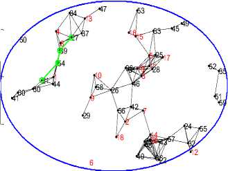
• D.    Experiment 1

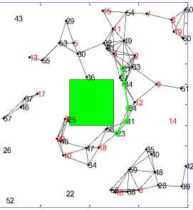
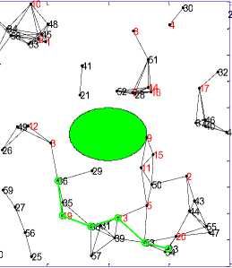
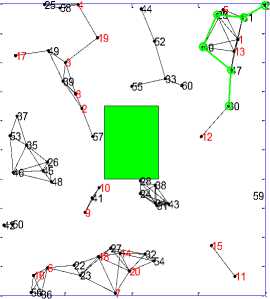
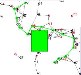
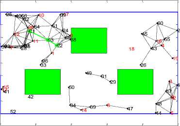
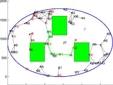
In this experiment we incorporated different shapes (Square, Rectangle, Square and Ellipse) of the obstacle in the simulation region to make the simulation realistic for CRN. In addition to it, number of PU’s and time allotted by PU to SU’s was also varied so as to show the need for CRN. Various snapshots of the simulation region are shown from Figure1 (a) to Figure1(d).

S= 22 D= 23 Duration= 17 Nodes 60

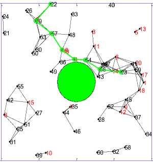
Figure 1(a). Circular obstacle

S= 21 D= 23 Duration= 26 Nodes 60

500         1000        1500        2000

Figure 1(b). Square obstacle

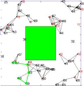
S= 23 D= 36 Duration= 17 Nodes 60

0          500        1000        1500        2000

Figure 1(c). Ellipse obstacle

D.1. PDR Comparison

Figure 1.1 to Figure 1.4 shows the graphs for different shapes of the obstacle. From the results following inference can be drawn:

• By increasing the PU Concentration and Increasing the PU activation time the value of PDR increases significantly.

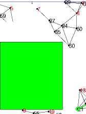
S= 21 D= 30 Duration= 40 Nodes 60

500         1000         1500        2000

• •    The value of the PDR with obstacles is found to be highest for circular shaped obstacle.

• •    The slope of the graphs in case of circular region is highest.

• •    PDR curve for the Ellipse and square regions are approximately same. the PDR curve for ellipse approaches the PDR curve for the square region on the cost of increased Hop Count

• •    PDR in case of rectangular obstacle is least, which is due to increase in the Hop Count and Path length.

• •    Slope of curves is least in the case of rectangular obstacle.

• •    Fluctuations in the PDR curve for Rectangular obstacle are maximum i.e. longer the length of path more is the probability of break in the path.

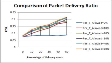
Figure 1.1. Impact on PDR in Circular obstacle situation

D.2 Hop Count Comparison

The following inference can be drawn from the graphs:

• •     Hop count value is maximum in case of

rectangular shaped obstacle.

• •      In comparison to other shape of the obstacle the

fluctuations in value for rectangular obstacle is maximum.

• •     The slope for Hop Count in case of ellipse and

square shapes is approximately same.

• •     As the concentration of PU nodes is increased

from 0 to 10%, the variation in the value of hop count is negligible.

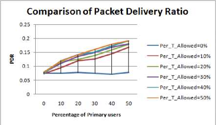
Figure 1.2. Impact on PDR in Square obstacle situation

Figure 1(d). Rectangle obstacle

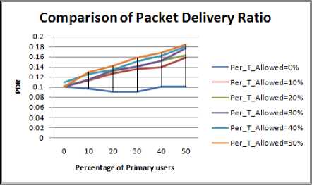
Figure 1.3. Impact on PDR in Elliptical obstacle situation

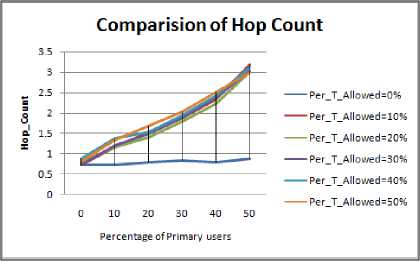
Figure 1.6. Impact on Hop Count in square obstacle situation

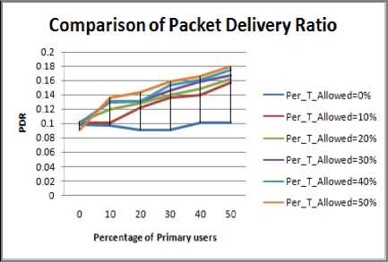
Figure 1.4. Impact on PDR in Rectangle obstacle situation

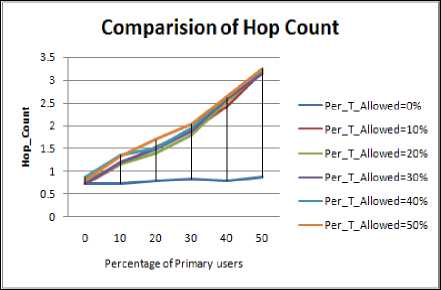
Figure 1.7. Impact on Hop Count ellipse obstacle situation

D.3. Path optimality comparison

Figure 1.9 to Figure 1.12 shows the path optimality values for different shape of the obstacle.

The following inference can be obtained about path optimality values:

• •    For all the shapes of the obstacles it can be seen that path length increases with increase in number of PU users.

• •    Maximum value of Path Optimality is obtained in the case of Rectangular obstacle. Thus it shows that in case of rectangular obstacle the path will not be reliable and hence its PDR value will be lesser in comparison to other shape of the obstacle.

• •    The fluctuations in case of rectangular and elliptical shape obstacles are greater as more is the path length more will be the likelihood of path break.

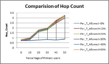
Figure 1.5. Impact on Hop Count in Circular obstacle situation

• E.    Analysis of Experiment 1

It can be seen from the Table 2 that best results are obtained in case of circular obstacle followed by square, ellipse and then rectangle. The reason for the same is the symmetry of the obstacle. As it is well known fact that “symmetry leads to stability” .Symmetry can be measured in terms of lines of symmetry i.e. a line that divides the figure in to two congruent parts.

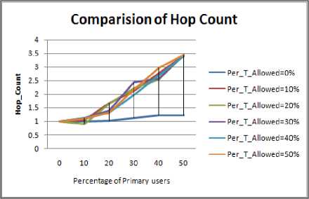
Figure 1.8. Impact on Hop Count in rectangle obstacle situation

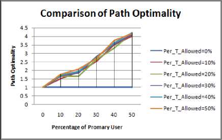
Figure 1.9. Impact on Path Optimality in Circular obstacle situation

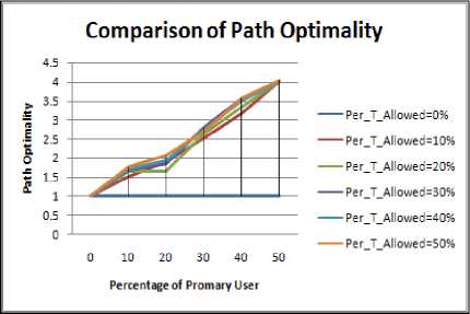
Figure 1.10. Impact on Path Optimality in square obstacle situation

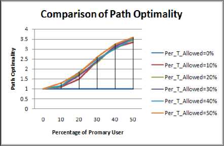
Figure 1.11. Impact on Path Optimality in elliptical obstacle situation

The obstacle shapes having more number of lines of symmetry will offer less hindrance. As observed in Table 2, Circular shape has highest lines of symmetry, while Ellipse and rectangle shapes have least number of lines of symmetry, consequently the hindrance in Elliptical and rectangular shapes will be maximum. This implies that the results of elliptical and rectangular obstacle should be same but the periphery of the rectangular shape obstacle is greater in comparison to elliptical shape. This leads to greater obstruction offered by the rectangular shape. Hence we can say that the results of hop count are in the increasing order of circle, square, ellipse and rectangular obstacle.

• F.    Experiment 2

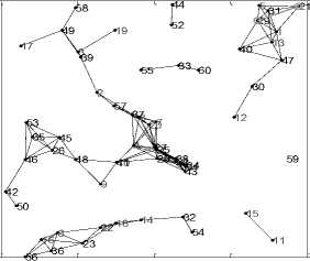
In this experiment we consider different type of obstacle such as river and Mountain. The former type obstacle i.e., river type will restrict the movement of nodes but the packets can be exchanged between the nodes present on either side of the river as also evident in the snapshot. On the other hand mountain type obstacle not only restricts the node movement but also cuts the communication otherwise possible between the nodes lying that are within the transmission range of each other.

Following Inference can be drawn from the Figure 2.1 and Figure 2.2

• •      In case of river type obstacle the PDR value is

higher in comparison to its value in mountain type obstacle.

• •     Increased fluctuation in PDR value for

mountain type obstacle due to longer path lengths.

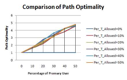
Figure 1.12. Impact on Path Optimality in Rectangular obstacle situation

Table 2: Overall Comparison of Experiment 1

Performance Metrics V -> Shape of Obstacle	Circle	Square	Ellipse	Rectangle
Lines of	Infinit	4	2	2
Symmetry	e
PDR	0.08	0.07	0.08	0.09
Min	0.21	0.19	0.18	0.18
Max
Path
Optimality
Min	1	1	1	1
Max	4.15	4.05	3.4	4.5
Hop count
Min	0.78	0.71	0.74	0.73
Max	3.25	3.11	3.14	3.44

S= 22 D= 28 Duration= 4 Nodes 60

1600 21

600 3

1000 x

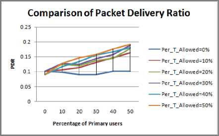
Figure 2.2. Impact on PDR in River type obstacle situation

Figure 2(a). Mountain type obstacle

S= 22 D= 23 Duration= 21 Nodes 60

1800 24

x

39 10

F.2. Hop Count Comparison

Figure 2.3 and Figure 2.4 show the hop count comparison for different types of the obstacles. The following inference can be drawn:

Comparisionof Hop Count

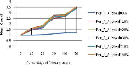
Figure 2.3. Impact on Hop Count in Mountain type obstacle situation

Figure 2(b). River type obstacle

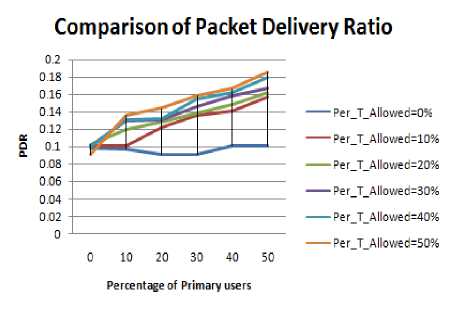
Figure 2.1. Impact on PDR in Mountain type obstacle situation

• •    The value of Hop Count is large for mountain type obstacle in comparison to river type obstacle as observed in Figure 2.3 and Figure 2.4.

• •    In case of mountain type obstacle the hop count value is consistently increasing for all values of PU, but in case of river type obstacle it is not so for the beginning concentration of PU(0 to 10%).

Comparisionof Hop Count

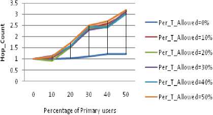
Figure 2.4. Impact on Hop Count in River type obstacle situation

reliable in comparison to mountain type obstacle.

Therefore the value of PDR is high in river type obstacle.

F.3. Path Optimality Comparison

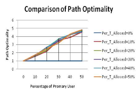
Figure 2.5. Impact on Path Optimality in Mountain type obstacle situation

Table 3: Overall Comparison of Experiment2

Performance Metrics Type of Obstacle	Mountain	River
PDR Min	0.09	0.09
Max	0.18	0.19
Path Optimality Min	1	1
Max	4.8	4.2
Hop count Min	1.18	0.94
Max	3.53	3.18

Comparison of Path Optimality

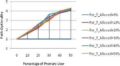
Figure 2.6. Impact on Path Optimality in River type obstacle situation

• •     In the mountain type obstacle deployment, the

maximum value of Path Optimality is greater as the paths formed will be longer due to presence of obstacles.

• •      Fluctuations in the River type are more as paths

formed are both around the obstacle as well as through the obstacle.

• •      Fluctuations in the mountain type are less as

paths formed will be around the obstacle only.

• G.    Analysis of experiment 2

Before discussing its analysis we would like to give some brief facts as follows:

• •     More is the path length higher are the chances

of path breakage

• •      A reliable path will certainly have more value

of PDR as its path length or hop count shall be small

The experimental result shows that in case of mountain the value of hop count is greater in comparison to river type obstacle since mountain type obstacle not only restricts node movement but also reduces effective transmission range of nodes i.e. it restricts the direct line of sight communication (see Figure 2(a)). As discussed the river type obstacle has lower value of path length hence path will be quite

• H.    Experiment 3

In this experiment an effort has been made to find impact of varying obstacle size on performance of CRN is observed. For this purpose a square obstacle is taken and its size is varied from 5% to 20% of the size of simulation region with step size of 5%. Figure 3(a) to Figure 3(d) gives the snapshot for varying size of obstacle.

S= 22 D= 28 Duration= 9 Nodes 60

1600 21

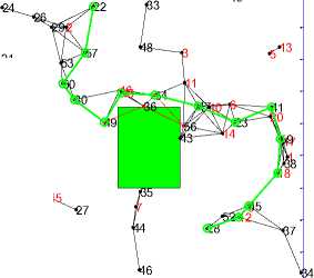
Figure 3(a). Size of obstacle 5%

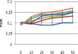
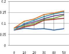
H.1. PDR Comparison

For this experiment we have considered mountain type obstacle. Figure 3.1 to Figure 3.4 displays the Variation in the value of PDR for different size of obstacle, with increase in concentration of Primary users. The following inferences can be drawn from the results.

• •    As the size of the obstacle increases the effective transmission range of nodes decreases therefore the value of PDR decreases. It is also observed that the maximum value of PDR among all the cases is highest for 5% size of obstacle.

• •    When the conditions of PU concentration and PU activation time are subjected; response is maximum for 5 % obstacle size case.

  y  yy

  
  
  

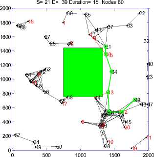
  Figure 3(b). Size of obstacle 10%

  
  
  
  

  S= 21 D= 50 Duration= 4 Nodes 60

  

  1000        1500        2000

  
  

  Figure 3(c). Size of obstacle 15%

  
  
  
  

  S= 21 D= 37 Duration= 11 Nodes 60

  
  
  

  500         1000        1500

  
  
  
  
  

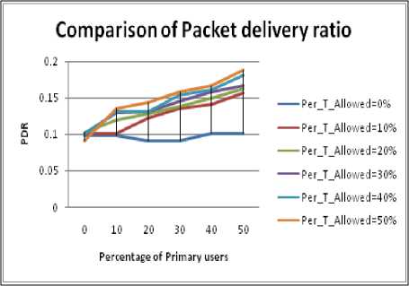
  Figure 3.1. Impact on PDR for 5% size obstacle situation

  
  
  

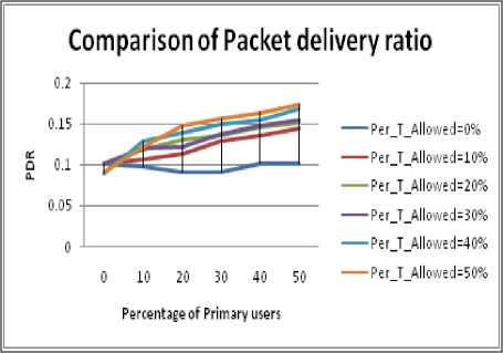
  Figure 3.2. Impact on PDR for 10% size obstacle situation

  
  

  Comparison of Packet delivery ratio

  
  
  

  — Per T Allowe d=50%

  ---PerJ_Allowed=5u%

  ---Per_T_AllowetMO%

  ----Pe r_T_Allowe d=0%

  ---PerJ_Allow;d=lu%

  — Per_T_Allowed=20%

  Percentage of Primary users

  
  

Figure 3(d). Size of obstacle 20%

Figure 3.3. Impact on PDR for 15% size obstacle situation

H.2. Hop Count Comparison

Figure 3.5 to Figure 3.8 show the impact on Hop Count for varying size of obstacle with increase in PU concentration. Following inference can be drawn:

• •    It can be easily seen that maximum hop count as well as path optimality value among all cases is largest for 5% size. On analysis it was found that the successful path formed in case of 20%,15% and 10% size of obstacles were quite low since the obstacle free

region that can be used for communication reduces as a result of which the value of hop count further reduces.

• •    Fluctuations in the values in the graphs are due to the randomness in the deployment of nodes in the simulation region.

• •    Little variations is observed for 0 to 20 % of nodes in values of Hop Counts in the graph for 20 % size of obstacle upto 20%.

Comparison of Packet delivery ratio

Q

----Per_T_Allowed=0%

----Per_T_Allowed=10%

----Per_T_Allowed=20%

---Per_T_Allowed=30%

----P e r_T_A 11 owe d=40%

----Per_T_Allowed=50%

Percentage of Primary users

Figure 3.4. Impact on PDR for 20% size obstacle situation

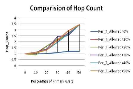
Figure 3.5. Impact on Hop Count for 5% size obstacle situation

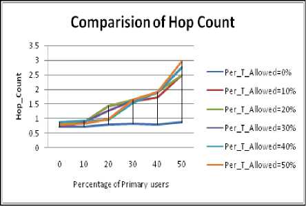
Figure 3.6. Impact on Hop Count for 10% size obstacle situation

H.3. Path Optimality Comparison

Figure 3.9 to Figure 3.12 shows the impact on path optimality for varying size of obstacle with rise in PU concentration. Following inference can be drawn:

• •    The maximum value of Path Optimality is obtained in case of 5% obstacle size. The reason for the same has been discussed above.

• •    For 15% and 20% size of obstacles, hop count change is negligible when PU concentration is raised from 10% to 20%.

• •    For 20% size obstacle change in the Hop Count value is small when PU concentration is raised from 30% to 40%.

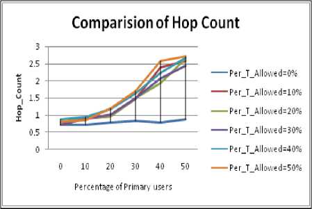
Figure 3.7. Impact on Hop Count for 15% size obstacle situation

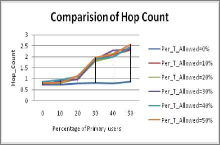
Figure 3.8. Impact on Hop Count for 20% size obstacle situation

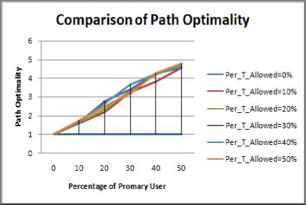
Figure 3.9. Impact on Path Optimality for 5% size obstacle situation.

• I.    Analysis of Experiment 3

The overall comparison of the performance metrics with the variation in size of obstacle is shown in Table 4.

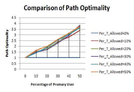
Figure 3.10. Impact on Path Optimality for 10% size obstacle situation.

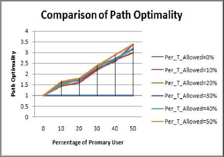
Figure 3.11. Impact on Path Optimality for 15% size obstacle situation.

Table 4: Overall Comparison of Experiment 3

Performance Metrics Size of Obstacle  —► 1	5%	10%	15%	20%
PDR Min	0.09	0.089	0.08	0.08
Max	0.18	0.17	0.16	0.15
Path Optimality Min	1	1	1	1
Max	4.8	3.9	3.5	3.1
Hop count Min	1.01	0.86	0.71	0.73
Max	3.49	3.05	2.72	2.56

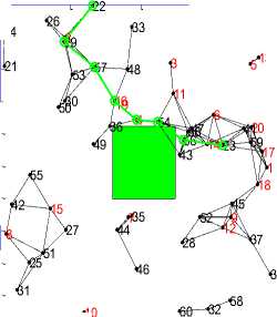
• J.    Experiment 4

In this experiment an effort has been made to find the Impact on the performance metrics by changing the shapes of the simulation region. In addition to it we also incorporated obstacles to evaluate the network performance. Figure 4(a) to Figure 4(h) shows the snapshots of the experiment performed.

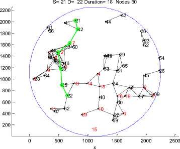
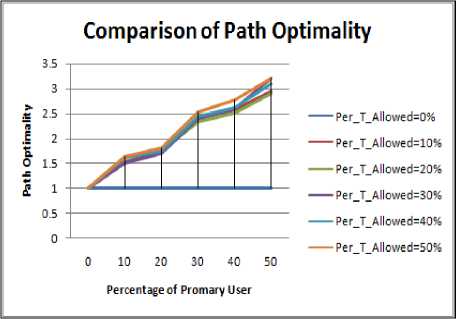
Figure 3.12. Impact on Path Optimality for 20% size obstacle situation

Figure 4(a). Circular shape without obstacle

S= 21 D= 23 Duration= 7 Nodes 60

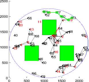
Figure 4(b). Circular shape with obstacle

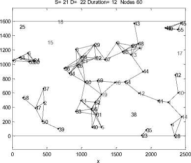
Figure 4(c). Rectangle shape without obstacle

S= 21 D= 27 Duration= 13 Nodes 60

500       1000       1500       2000       2500

x

Figure 4(g). Elliptical region without obstacle

yy

S= 21 D= 22 Duration= 16 Nodes 60

1000         1500         2000        2500

x

Figure 4(d). Rectangle shape with obstacle

S= 22 D= 25 Duration= 12 Nodes 60

500       1000       1500       2000      2500

x

S= 21 D= 29 Duration= 21 Nodes 60

x

Figure 4(h). Elliptical region with obstacle

Figure 4 (e). Square region without obstacles

J.1 PDR Comparison

Following inferences about PDR can be drawn from Figure 4.1 to 4.8

•     In case of idealistic scenario i.e. in absence of obstacle the value of PDR is comparatively higher for all the shapes of the periphery. This shows that idealistic results are quite different from realistic ones. Thus before choosing any routing protocol the geographical shape of the region should be considered to have better picture of realistic situation.

0 0

S= 21 D= 26 Duration= 6

Nodes 60

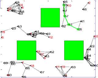
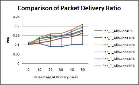
Figure 4.1. Impact on PDR in circular boundary without obstacle situation

Figure 4 (f) Square region with obstacle

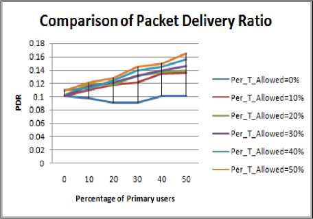
Figure 4.2. Impact on PDR in circular boundary with obstacle situation

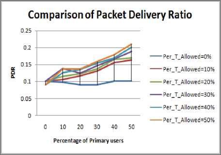
Figure 4.5. Impact on PDR in square boundary without obstacle situation

• •    Circular shape region has highest value of PDR value due to symmetry in deployment of nodes in circular region followed by square, rectangle and then elliptical peripheries.

• •    Change in the PDR when PU concentration is changed from 0% to 10 to 20% is quite small in scenario having obstacle.

  

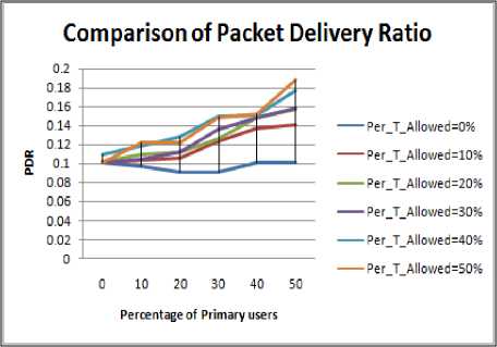
  Figure 4.6. Impact on PDR in square boundary with obstacle situation

  
  
  

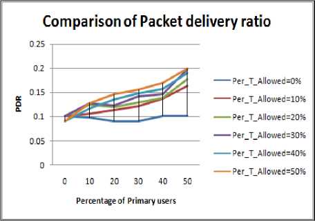
  Figure 4.3. Impact on PDR in Rectangular boundary without obstacle situation

  
  
  

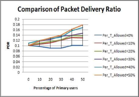
  Figure 4.4. Impact on PDR in Rectangular boundary with obstacle

  
  
  

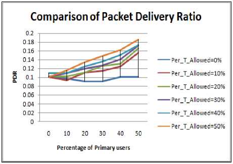
  Figure 4.7. Impact on PDR in Elliptical boundary without obstacle situation

  
  
  

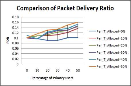
  Figure 4.8. Impact on PDR in Elliptical boundary with obstacle situation

  
  
  

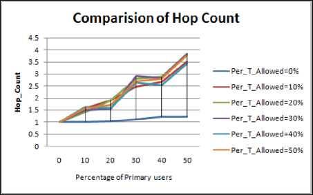
  Figure 4.11. Impact on Hop Count in Rectangular boundary without obstacle situation

  
  

J.2 Hop Count Comparison

Figure 4.9 to Figure 4.16 shows the hop count for different shape of the periphery, following inference can be drawn:

• •    As discussed the circle has maximum value of PDR therefore its hop count must be least as also depicted from our results.

• •    As discussed the elliptical shape of the periphery and rectangular shape has same value of line of symmetry hence the results of hop count are nearly same.

• •    The realistic results are quite different from the idealistic ones as also proven above.

  

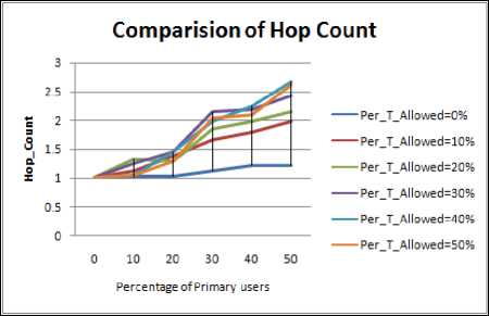
  Figure 4.12. Impact on Hop Count in Rectangular boundary with obstacle situation

  
  
  

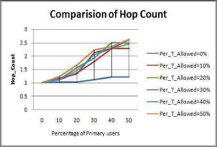
  Figure 4.9. Impact on Hop Count in circular boundary without obstacle situation

  
  
  

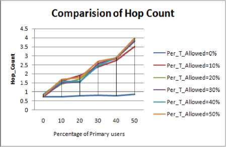
  Figure 4.13. Impact on Hop Count in square boundary without obstacle situation

  
  
  

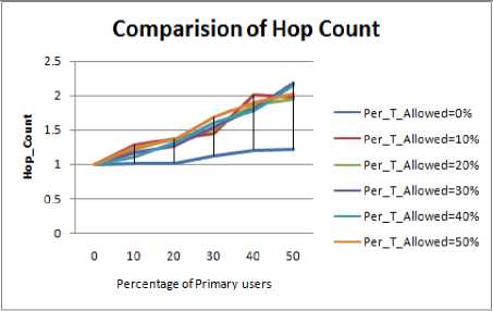
  Figure 4.10. Impact on Hop Count in circular boundary with obstacle situation

  
  
  

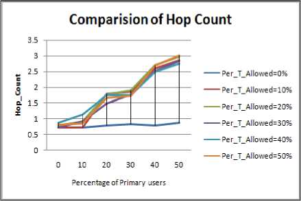
  Figure 4.14. Impact on Hop Count in square boundary with obstacle situation

  
  
  

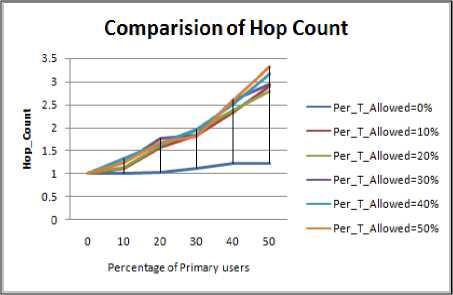
  Figure 4.15. Impact on Hop Count in Elliptical boundary without obstacle situation

  
  
  

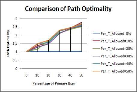
  Figure 4.18. Impact on Path Optimality in circular boundary with obstacle situation

  
  
  

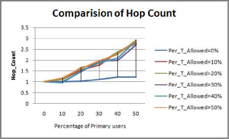
  Figure 4.16. Impact on Hop Count in Elliptical boundary with obstacle situation

  
  
  

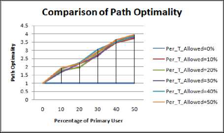
  Figure 4.19. Impact on Path Optimality in Rectangular boundary without obstacle situation

  
  

J.3. Path Optimality Comparison

Figure 4.17 to Figure 4.24 shows the path optimality for different shape of the periphery, Following inference can be drawn:

• •    As discussed the circle has maximum value of PDR therefore its path length and hop count must be least as also depicted from our results.

• •    As discussed the elliptical shape of the periphery and rectangular shape has same value of line of symmetry hence the results of hop count are nearly same..

• •    The realistic results are quite different from the idealistic ones as also proven above.

  

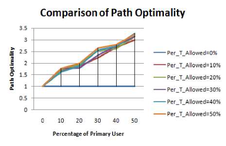
  Figure 4.20. Impact on Path Optimality in Rectangular boundary with obstacle situation

  
  

  Comparison of Path Optimality

  
  
  

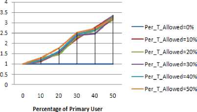
  Figure 4.17. Impact on Path Optimality in circular boundary without obstacle situation

  
  
  

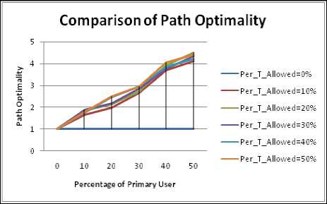
  Figure 4.21. Impact on Path Optimality in square boundary without obstacle situation

  
  
  

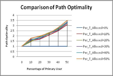
  Figure 4.22. Impact on Path Optimality in square boundary with obstacle situation

  
  
  

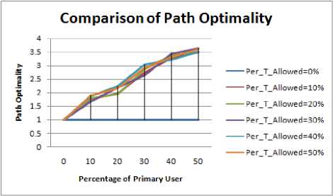
  Figure 4.23. Impact on Path Optimality in Elliptical boundary without obstacle situation

  
  

K. Analysis of Experiment 4

From this experiment it can be easily seen that if the geographical shape is circular all the performance metrics proves to be the best. The reason behind this is the fact the circular region has infinite lines of symmetry. For the other shape i.e. square which has four lines of symmetry has the best performance when compared with rectangle and ellipse. The other two shapes have same lines of symmetry that’s why their results are nearly same as also shown in Table5.

• IV. CONCLUSION

In this paper an effort has been made to make the scenario realistic for CRN. Following are the outcomes of this paper that can prove very much beneficial for researchers:

• (1)    Realistic results obtained are quite different from ideal ones as shown. Thus they cannot be used in actual scenarios of deployment of CRN.

• (2)    Before choosing any protocol for simulations the geographical shape of the network must be taken into consideration since different shape of the simulation region have different impact on performance of routing protocols.

• (3)    The behaviour of routing protocol is quite different in the simulation region having different type of obstacles.

The paper also shows how crn can solve our network scarcity problem.

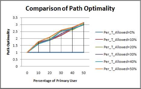
Figure 4.24. Impact on Path Optimality in Elliptical boundary with obstacle situation

Table 5: Overall Comparison of Experiment 4

Performance Metrics Shape of Boundary■>		Circle Without With		Square Without With		Ellipse		Rectangle
						Without Obst .	With Obst.	Without Obst.	With Obst.
		Obstacle O	bstacle
				Obst .	Obst.
Lines of Symmetry		Infinite		4		2		2
Min		0.11067	0.10131	0.10131	0.10067	0.10067	0.10965	0.09912	0.91233
PDR	Max	0.21164	0.16545	0.21007	0.18797	0.18523	0.16062	0.20076	0.17864
Path	Min	1	1	1	1	1	1	1	1
Optimality	Max	3.21	2.65	4.4	3.48	3.62	3.14	3.98	3.24
Min		1.051	1.012	0.86705	0.8056	1.023	0.923	0.923	1.011
Hop count	Max	2.632	2.023	3.853	3.0091	3.326	2.930	3.767	2.618