Transfer Subspace Learning Model for Face Recognition at a Distance

Автор: Alwin Anuse, Nilima Deshmukh, Vibha Vyas

Журнал: International Journal of Image, Graphics and Signal Processing(IJIGSP) @ijigsp

Статья в выпуске: 1 vol.9, 2017 года.

Бесплатный доступ

Many machine learning algorithms work under the assumption that the training and testing data are drawn from the same distribution. However, in practice the assumption might not hold. Transfer subspace learning algorithms aims at utilizing knowledge gained in source domain to learn a task in target domain. The main objective of this work is to apply transfer subspace learning framework on face recognition task at a distance. In this paper we identify face recognition at distance as a transfer learning problem. We show that if the face recognition task is modeled as transfer learning problem, the overall classification rate is increased significantly compared to traditional brute force approach. We also discuss a data set which is unique and meant to advance this research. The novelty of this work lies in modeling face recognition task at distance as a transfer subspace learning problem.

Еще

Face recognition, Transfer subspace learning, KNN, independent and identically distributed

Короткий адрес: https://sciup.org/15014155

IDR: 15014155

Текст научной статьи Transfer Subspace Learning Model for Face Recognition at a Distance

Published Online January 2017 in MECS

Many Machine learning algorithms assume that the training and testing data belong to same feature space and the same distribution [1]. However, in practice this is not the situation. The data may belong to different distribution, for e.g. in face recognition application, the face images may be taken under different illumination conditions, pose changes, expression changes etc. It is very difficult to maintain the same environmental conditions at the time of testing which were present during image acquisition for training task. The training data might not be available at the same time. The system has to be retrained if the data distribution changes. In many situations, it is expensive or impossible to collect the training data and retrained the system [1]. In such situations transfer learning approach is useful.

Transfer learning approach stores knowledge at the time of training and uses it at the time of testing. Transfer learning uses both labeled and unlabeled samples, similar to semi supervised learning. In semi supervised learning, the training and testing samples are usually independent and identically distributed (i.i.d) [3] and thus, the distribution of the training samples is consistent with that of testing samples . When labeled samples are available, auxiliary information is utilized in transfer learning. The auxiliary information may be in the form of sharing features from auxiliary tasks [4], data from auxiliary domains [5]. By assuming that both source and target modality are accessible in the training phase, knowledge is transferred in the multimodal transfer learning. For e.g. in Face recognition one might have near infrared images as source and visible images as target modality [11]. Liu Yang and Etal showed that text-to-image transfer learning can be done in noisy environment [12]. Transfer learning is been used in regression, classification and unsupervised learning [13].

Lot of research is going on developing Face recognition algorithms which are invariant to pose [14], expressions [15], illumination [16] and distance [17]. In this paper we have addressed the problem of face recognition at a distance. The contribution of this research work are:

a. Use of transfer learning model for face recognition at a distance
b. Novel dataset which is developed and meant to advent this research.

II. Related Work

Transfer subspace learning has advanced considerably since the work of Si Si et.al (2010), which we use our baseline. In their research [2], they have proposed Bregman divergence based regularization for transfer subspace learning which boost performance when training and testing samples are not independent and

identically distributed. They performed their experiments on public datasets, e.g. YALE [6], FERET [7] etc. None of the dataset is meant for distance invariance experimentation .The dataset described by us meant exclusive for the experimentation on distance invariance. Many researchers have applied subspace learning to small scale applications like text classification , sensor network based localization, image classification [4-5].Various application of transfer subspace learning are explained in [10].

III. Transfer Subspace Learning Framework

Let there be m training and n testing samples, which belongs to a high dimensional space RS. Any subspace learning algorithm can find a low dimensional space Rs, wherein we get separation among samples from different classes. If x is the feature vector such that xϵ RS, then there exists linear function y = VT x, wherein Vϵ RSxs and yϵ Rs. The linear function can be obtained from

V =argmin F ( V ) (1)

Subject to V^T V = I. The objective function F(V) is designed to minimize the classification error. The traditional subspace learning framework (1) will perform well only if training and testing samples are independent and identically distributed. However, sometimes the distribution of the training samples P m and that of testing samples P n is different. Under such conditions, the subspace learning framework (1) will fail. To address this problem one can use Bregman divergence-based regularization D_V(P_m‖ P_n) , which measures the distance between the distributions of the training and testing samples in a projected subspace V. Accordingly , the framework in (1) is modified as given in eqn (2)

V =arg F ( V )+ a D_v ( Pm ‖ Pn ) (2)

Subject to V^T V = I. Regularization parameter α controls the trade-off between F(V) and D V (P m ‖ P n ). Gradient descent algorithm can be used to obtain the solution of (2), i.e.

V ( new )= V ( old. )-

μ ( аг ⁽ ) ₊ a ( Pm ‖ Pn ⁾ ) (3)

\ dV dV / v '

Where µ is the learning rate.

A. Framework of Transfer Subspace learning(TSL) applied to Principal Component Analysis (PCA)

There are many popular subspace learning algorithms like unsupervised principle component analysis (PCA), supervised linear discriminant analysis (LDA) and locality preserving projection (LPP). Projection of data by linear transformation technique is a key concept in all these algorithms.

PCA projects the high dimensional data to lower dimensional space by capturing maximum variance [8].

PCA projection matrix maximizes the trace of the total scatter matrix

V=argmaxtr (VT AV)(4)

Subject to VT V = I. A is the autocorrelation matrix of training samples. F(V) of PCA is given by (5)

F(V)= -tr (VT AV)(5)

( V-)= -2AV(6)

IV. Algorithm

In subspace learning algorithm, high dimensional data is projected into a low dimensional subspace preserving specific statistical properties. Fisher linear discriminative analysis (FLDA), minimizes the trace ratio between the within class and between the class scatter [18]. Locality preserving projection (LPP) preserves the local geometry of samples [19]. Principal component analysis (PCA) is an unsupervised method that projects the high dimensional data to lower dimensional space by capturing maximum variance. PCA steps are explained in section IV (A). If the training and testing samples are not independent and identically distributed, PCA gives very poor performance. Transfer principal component analysis (TPCA) learning algorithm takes into account the distribution difference between the training and testing samples. TPCA steps are explained in section IV (B).

A. PCA steps

Step 1 Subtract the mean

From all the samples of training set, subtract the mean from each of the data dimensions.

Step 2 Calculate the covariance matrix

Step3 Calculate the eigen vectors and eigen values of the covariance matrix

Step 4 Choose components and form a feature vector

The eigen vector with the highest eigen value is the principle component of the data set. Feature vector is constructed by taking the eigen vectors that we want to keep from the list of eigen vectors.

Step5 Deriving new data set.

New data vector y = V x, where x is old vector and V is the transformation matrix of PCA projection matrix made of eigen vectors.

B. TPCA ( Transfer Principle Component Analysis) steps

Step 1 Add new samples to the old data set.

Step 2 Choose the initial guess V

V learned from F(v) is a good initial guess.

Step 3 Choose the learning rate µ and regularization parameter α.

These values should be greater than zero but less than or equal to one.

Step 4 Find the autocorrelation matrix of the samples in the dataset.

Step 5 Update

Equation (3) subject to VTV =I.

V. Dataset

For the experimentation, we constructed our own database. By varying the distance between camera and subject, the database was prepared. The distance was varied in steps of 15 cm .We referred to distance of 15 cm a scale S1, 30 cm as S2 and 120 cm as S 8 etc. The database contains 10000 images that includes 50 subjects .For every subject 25 images at a distance of 15 cm were taken. The database is under construction. Sample images are shown in Fig1.

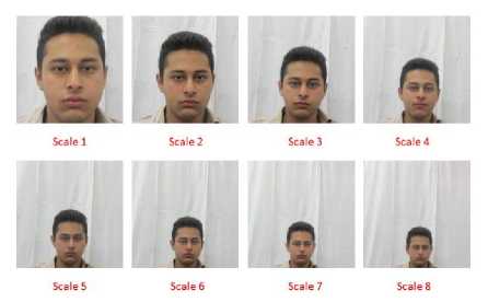
Fig.1. Sample Images in Database

VI. Experimentation

KNN (K nearest Neighbors) [9] classifier is been trained with PCA features for different subspaces and the classification rates on same scale and cross scale is found. KNN classifier is also been trained and tested with Transfer PCA features for different subspace dimensions. The results of the same are shown in table 1-6. Brute force approach is also used to train KNN. In Brute force approach the KNN is trained with samples taken at two distances. Results of brute force method are shown in table 7.

Regularization parameter was heuristically set to 0.5. The learning rate parameter was initially set to 1 and then decreased to 0.3. The nearest neighbor rule is used for classification. It is essential to have one reference image for each testing class. In the training stage no labeling information is available. The labeling information of reference images is available only for classification in the testing stage. Distance between every reference image and testing image is calculated for predicting the label of the testing image as that of the nearest reference image.

VII. Results

Table 1. PCA with 10 x 10 subspace

KNN classifier trained with PCA Features with 10 X 10 subspace dimensions
Training	S1	S2	S3	S4	Testing S5	S6	S7	S8
S1	75	10	9	15	4	8	9	7
S2	17	78	18	12	11	8	10	12
S3	10	10	74	18	11	17	17	12
S4	12	13	9	76	8	9	12	13
S5	5	6	7	22	78	24	17	12
S6	15	13	15	10	19	79	22	15
S7	13	15	12	11	10	13	78	13
S8	10	6	12	11	15	25	26	88

Table 2. TPCA with 10 x 10 subspace

KNN classifier trained with TPCA Features with 10 X 10 subspace dimensions
Training	S1	S2	S3	S4	Testing S5	S6	S7	S8
S1	78	60	75	70	80	78	85	84
S2	88	82	84	85	75	80	82	85
S3	45	90	91	90	90	85	88	85
S4	40	95	95	90	78	92	92	92
S5	46	55	72	72	82	85	84	85
S6	50	95	95	95	97	88	97	96
S7	48	90	83	84	86	82	82	80
S8	45	92	93	92	93	94	94	95

Table 3. PCA with 20 x 20 subspace

KNN classifier trained with PCA Features with 20 X 20 subspace dimensions
Training	S1	S2	S3	S4	Testing S5	S6	S7	S8
S1	82	14	4	5	8	9	12	12
S2	14	80	18	12	16	10	12	13
S3	14	16	80	20	18	18	10	15
S4	7	10	13	85	16	10	12	10
S5	11	10	8	9	87	10	11	16
S6	12	10	13	12	10	78	12	10
S7	18	12	14	18	17	16	81	12
S8	13	18	15	16	8	9	10	75

Table 4. TPCA with 20 x 20 subspace

KNN classifier trained with TPCA Features with 20 X 20 subspace dimensions
Training	S1	S2	S3	S4	Testing S5	S6	S7	S8
S1	85	92	90	75	84	98	98	97
S2	97	82	75	97	48	94	97	98
S3	50	55	83	45	46	75	96	88
S4	82	96	47	86	56	98	86	87
S5	42	45	49	55	78	82	98	97
S6	90	85	55	97	90	80	97	58
S7	90	84	54	97	98	82	84	45
S8	86	88	95	68	97	97	98	78
		Table 5. PCA with 30 x 30 subspace
KNN classifier trained with PCA Features with 30X30 subspace dimensions
Training					Testing
	S1	S2	S3	S4	S5	S6	S7	S8
S1	74	5	18	4	6	5	4	3
S2	10	70	8	7	6	5	10	7
S3	6	8	72	9	10	6	8	11
S4	8	9	10	76	10	9	8	7
S5	6	5	4	4	72	10	11	12
S6	10	9	8	6	12	73	10	11
S7	12	14	15	16	15	16	70	18
S8	18	17	10	11	13	12	11	72

Table 6. TPCA with 30 x 30 subspace

KNN classifier trained with TPCA Features with 30X30 subspace dimensions
Training	S1	S2	S3	S4	Testing S5	S6	S7	S8
S1	78	45	53	57	62	60	61	59
S2	66	65	64	66	62	61	69	68
S3	40	65	64	62	61	53	54	53
S4	42	58	62	67	68	63	62	60
S5	39	44	60	61	65	68	62	60
S6	46	70	68	68	62	66	62	53
S7	42	70	63	66	65	62	61	68
S8	40	68	63	62	66	62	61	64

Table 7. PCA with 20 x 20 subspace (Brute force method)

KNN classifier trained with PCA Features with 20X20 subspace dimensions (Brute Force
	Method)
Training	S1	S2	S3	S4	Testing S5	S6	S7	S8
S1- S2	70	72	10	13	14	9	4	8
S2- S3	10	74	72	14	6	9	8	10
S3- S4	10	7	71	75	9	10	8	10
S4- S5	5	10	4	73	72	9	8	10
S5 –S6	11	10	12	8	70	72	4	6
S6 –S7	7	8	10	5	6	72	71	8
S7- S8	4	7	9	8	6	5	71	70
S8- S1	70	2	10	6	5	8	9	70

Scale

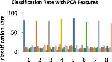
Fig.2. Plot of Classification rates with PCA features for 20x20 subspace

Classification rate with TPCA Features

ф го

о го

го

Scale

Fig.3. Plot of Classification rates with TPCA features for 20x20 subspace

VIII. Conclusion and Discussion

We have experimented using PCA with different subspace dimensions viz. 10x10, 20x20, 30x30, 40x40 and 50x50 .Results upto 30x30 dimensions are listed in this paper. We found that as the subspace dimensions increase, the correlation gets captured which results in the decrease of classification rate. The best results are available with 20x20 subspace dimensions as maximum variance is captured by PCA in that subspace dimension. The results of the same are shown in Fig 2 and Fig 3.

Список литературы Transfer Subspace Learning Model for Face Recognition at a Distance

Sinno Jialin Pan and Qiang Yang A Survey on Transfer Learning. IEEE Transactions on Knowledge and Data Engineering, 2010, vol 22, No 10.
Si Si and Dacheng Tao Bregman Divergence –Based Regularization for Transfer Subspace Learning . IEEE Transactions on Knowledge and Data Engineering, 2010, vol22, No 7.
M.Beklin, P.Niyogi and V.Sindhwani, Manifold Regularization: A Geometric Framework for Learning from Labeled and Unlabeled Examples. J.Machine Learning Research, 2006, 7:.2399-2434.
B.Zadrozny Learning and Evaluating Classifiers under Sample Selection Bias. Proc.21st International conference on Machine Learning, 2004, 114-121.
S.J.Pan, J.T. Kwok, and Q.Yang. Transfer Learning via Dimensionality reduction.Proceedings of 23rd national conference on Artificial intelligence, 2008, 677-682
P.N.Belhumeurb, J.P Hespanha, and D.J.Kriegman. Eigenfaces versus Fisherfaces: Recognition Using Class Specific Linear Projection," IEEE Transaction Pattern Analysis and Machine Intelligence, 1997, 19:711-720
P. J. Phillips, H. Wechsler, J. Huang, and P. Rauss. The FERET database and evaluation procedure for face recognition algorithms. Image Vis. Comput. J., 1998, vol. 16.5: 295–306.
Stan Z.Li and Anil K,.Jain . Handbook of Face Recognition, second Edition.Springer.
Desislava Boyadzieva George Gluhchev. Neural Network and KNN classifier for on line signature verification. Lecture Mnotes in Computer Science, 2014, 8897:198-206
Ming Shao Dmitry Kit Yun Fu. Generalized Transfer subspace learning through low rank constraint. Int J Comput Vis. 2014, 109:74-93.
Zheng Ming Ding, Ming Shao and Yun Fun, "Missing Modality Transfer Learning via latent low rank constraint" IEEE transactions on Image Processing, Nov 2015, vol 24, pp 4322-4334.
Li Yang, Liping Jing and Michael K Ng, " Robust and Non-negative Collective Matrix Factorization for Text–to-Image Transfer Learning", IEEE transactions on Image Processing, Dec 2015, vol 24, No 12, pp 4701-4714.
Zhaohong Deng, Yizhang Jiang, "Generalized Hidden-Mapping Ridge Regression, Knowledge-Leveraged Inductive Transfer Learning for Neural Networks, Fuzzy Systems and Kernel Methods", IEEE Transactions on Cybernetics, Dec 2014, vol 44, No 12, pp 2585-2599
Teddy Salan, Khan M Iftekharuddin, "Large Pose Invariant Face Recognition using feature based recurrent neural network", International Conference on Neural Network, 2012, DOI:10:1109/IJCNN.2010.6252795
H Ebrahim Pour- Komleh, V Chandran, S Sridharan, "Robustness to expression variations in fractal base face recognition", Sixth International Symposium on Signal Processing and its Applications, 2001, vol 1, pp 359-362
Horst Eidenberger, "Illumination Invariant Face Recognition by Kalman Filtering", Proceedings ELMAR 2006, DOI:10:1109/ELMAR.2006.329517
M.S.Shashi Kumar, K.S.Vimala, N.Avinash, "Face Recognition distance estimation from a monocular camera", IEEE conference on Image Processing, 2013, DOI 10:1109/ICIP.2013.6738729
Fisher RA, "The use of multiple measurements in taxonomic problems, Ann Evgen, 7(2), 1936, pp 179-188
He X, Niyogi P, "Locality preserving projections", Advanced Neural Information Processing System, 2003, pp 16:1-8
Belhumeur p, Hespanha J, Kriegman D, "Eigenfaces vs fisher faces: recognition using class specific linear projection, IEEE Trans Pattern Analysis and Machine Intelligence, 1997, 19(7), pp 711-720

Еще

Статья научная