Traveling Transportation Problem Optimization by Adaptive Current Search Method

Автор: Supaporn Suwannarongsri, Tika Bunnag, Waraporn Klinbun

Журнал: International Journal of Modern Education and Computer Science (IJMECS) @ijmecs

Статья в выпуске: 5 vol.6, 2014 года.

Бесплатный доступ

The adaptive current search (ACS) is one of the novel metaheuristic optimization search techniques proposed for solving the combinatorial optimization problems. This paper aimed to present the application of the ACS to optimize the real-world traveling transportation problems (TTP) of a specific car factory. The total distance of the selected TTP is performed as the objective function to be minimized in order to decrease the vehicle’s energy. To perform its effectiveness, four real-world TTP problems are conducted. Results obtained by the ACS are compared with those obtained by genetic algorithm (GA), tabu search (TS) and current search (CS). As results, the ACS can provide very satisfactory solutions superior to other algorithms. The minimum total distance and the minimum vehicle’s energy of all TTP problems can be achieved by the ACS with the distant error of no longer than 3.05%.

Еще

Traveling transportation problem, adaptive current search, metaheuristic optimization

Короткий адрес: https://sciup.org/15014653

IDR: 15014653

Текст научной статьи Traveling Transportation Problem Optimization by Adaptive Current Search Method

Published Online May 2014 in MECS

The traveling transportation problem (TTP) is one of the most intensively studied problems in computational mathematics and combinatorial optimization. The problem is to find an optimal tour for a traveling transportation wishing to visit each of a list of n cities exactly once and then return to the home city. Such optimal tour is defined to be a tour whose total distance (cost) is minimized. The TTP is considered as the class of the traveling salesman problem (TSP) which is one of the combinatorial optimization problems known as NP-complete [1, 2]. By literature, many algorithms and approaches have been launched to solve the TSP and TTP problems. Those algorithms can be classified into exact and heuristic approaches [3, 4] such as dynamic programming [5], branch-and-bound [6], branch-and-cut [7] and linear programming [8]. The heuristic methods could provide very satisfactory solutions of the problems possessing large amount number of cities. However, the optimum solution could not be guaranteed. Up to date, the metaheuristic optimization techniques have been applied to solve the TPS and TTP problems, for example simulated annealing (SA) [9], artificial neural network (ANN) [10], tabu search (TS) [11], genetic algorithms (GA) [12], scatter search [13], particle swarm optimization [14], ant colony optimization [15] and adaptive tabu search (ATS) [16].

The adaptive current search (ACS) is one of the most efficient metaheuristic optimization techniques. The ACS has been developed in 2014 [17, 18] as the modified version of the conventional current search [19,20] developed from the behavior of an electric current flowing through electric networks. The ACS has possessed the memory list (ML) and the adaptive radius (AR) mechanism. The ACS effectiveness has been improved to escaping from any local entrapment and to speed up the search process. The performance of the ACS over unconstraint and constraint optimization problems has been evaluated [17]. It was found in the previous work that the ACS outperforms GA, TS and CS and provides superior results which are very close to the optimal solutions for all benchmark tested functions. Moreover, the ACS has been applied to solve the real-world assembly line balancing (ALB) problems of a car factory according to energy resource management optimization context [18].

In this paper, the ACS is applied to solve real-world TTP problems of a specific car factory in sense of the energy resource management optimization context. Based on exactly optimal solutions, results obtained by the ACS will be compared with those obtained by three well-known metaheuristic optimization techniques, i.e. GA, TS and CS.

This paper consists of six sections. After an introduction provided in section 1, the problem formulation of TTP problem is illustrated in section 2. The ACS algorithms are briefly described in section 3. Application of the ACS to the TTP problems is explained in section 4. Results of the TTP problem solving are provided and discussed in section 5, while conclusions are given in section 6.

II. Traveling Transportation Problem

Formulation

The traveling transportation problem (TTP) can be considered as the traveling salesman problem (TSP) which has been firstly proposed as one of the mathematical problems for optimization in 1930s [2,3]. The problem is to find an optimal tour for a traveling salesman wishing to visit each of a list of n cities exactly once and then return to the home city. Such optimal tour is defined to be a tour whose total distance (cost) is minimized. This problem can be considered as the class of combinatorial optimization problems known as NP-complete.

By theory, the TSP (TTP) has been firstly proposed as one of the mathematical problems in 1800s by Harmilton and Kirkman [2, 3]. However, the general formulation of TSP has been firstly lunched based on the graph theory in 1930s [2, 3, 4]. Let G = ( V, E ) be a complete undirected graph with vertices V , | V | = n , where n is the number of cities, and edges E with edge length c ij for the- ij city ( i , j ). In this work, the symmetric TTP problems are focused so that c_i j = c j _i , for all cities ( i , j ). As the constrained optimization problem, the TTP problem formulations for minimization as expressed in (1) – (5). J in (1) is the objective function standing for the energy used for traveling. J will be minimized. Constraints (2) and (3) define a regular assignment problem, where (2) ensures that each city is entered from only one other city, while (3) ensures that each city is only departed to on other city. Constraint (4) eliminates sub tours. Constraint (5) is a binary constraint, where x_i j = 1 if edge ( i , j ) in the solution and x_i j = 0, otherwise.

Min J =∑∑cijxij(1)

i ∈ V j ∈ V

Subject to ∑xij = 1, i ∈ V(2)

j ∈ V , j ≠ i

∑xij =1, j∈V(3)

i ∈ V , i ≠ j

∑∑xij≤ I S I -1, ∀S⊂V,S=∅ i∈S j∈S xij = 0 or 1, i, j ∈V(5)

The difficulty of solving TTP is that sub tour constraints will grow exponentially as the number of city grows large. It is not possible to generate or store these constraints. Many applications in real-world could not provide optimal solutions. Therefore, several metaheuristic algorithms have been proposed to solve such the problems.

In sense of the energy resource management optimization context, optimized TTP problems can save the main energy consumption for transportation by any vehicle. Moreover, minimized distance of the TTP can provide the minimum supporting energies for breakage and maintenance, lubricant oil- and tire- changing and so forth. However, these energies are in the form of costs. They will be neglected in this work. The main energy used for transportation (W) of TTP problems can be yearly calculated in liter (l.) unit by (6), where E′ is the energy consumption (vehicle’s fuel) per unit of distance to be traveled and T stand for the numbers of traveling times in each year.

J × T

E ′

III. Adaptive Current Search Algorithms

Based on the principle of current divider in electric circuit theory, the current search (CS) was developed in 2012 [19, 20]. The CS possesses the exploration and exploitation properties. However, the search process of the CS may be trapped by any local solution. In addition, the search time consumed by the CS is depended on the numbers of search directions. In 2014, the modified version of the CS named the adaptive current search (ACS) has been proposed [17, 18]. The ACS possesses the memory list (ML) and the adaptive radius (AR) mechanism. By this fashion, the ML is used to escape from local entrapment caused by any local solution, while the AR is conducted to speed up the search process. The proposed ML consists of three levels: low, medium and high. The low-level ML is used to store the ranked initial solutions at the beginning of search process, the mediumlevel ML is conducted to store the solution found along each search direction, and the high-level ML is used to store all local solutions found at the end of each search direction. To perform its effectiveness, the ACS has been evaluated against benchmark unconstrained and constrained optimization problems [17]. Once compared with GA, TS and CS, it was found that the ACS shows the superior results to the conventional CS and other algorithms. The real-world application of the ACS over the ALB problems of a specific car factory according to energy resource management optimization has been successfully achieved [18]. The ACS algorithms can be represented by the pseudocode as shown in Fig. 1.

IV. Adaptive Current Search Application to Traveling Transportation Problems

This section presents the application of the ACS to the TTP problems of a specific car factory. Sammitr Motors Manufacturing Public Co., Ltd. [21], a car factory located in Samut Sakhon, Thailand, is considered as a case study of this work. It produces car and truck body parts, moulds and fixtures for auto makers such as HINO, ISUZU, MITSUBISHI and NISSAN. Many kinds of car and truck body parts under “Sammitr” trademark are assembled and delivered from this factory. Now, Sammitr need to solve its TTP problems. Regularly, it has oneregion to transport car and truck body parts. It is the Bangkok and nearby province region. However, Sammitr has a plan to expand transportation network for sending

Pseudo-code of ACS procedure

Initialize the search space = Ω, the memory lists (ML) Ψ = Γ = Ξ = ∅, the iteration counter i = j = k = l = 1, the maximum search iteration in each direction Imax, the maximum allowance of solution cycling jmax, the number of initial solutions (feasible directions of currents in network) N, number of neighborhood members n, the maximum objective function value ε for AR, and the search radius R.

while ( i < N ) do // generate search directions Generate initial solutions X i randomly within Ω; Evaluate f ( X i ) via the objective function; Rank X i giving f ( X i ) from min to max values ( X 1 gives the min, while X N gives the max objective function values); Store ranked X i into Ψ;

end_while while (k ≤ N) or the TC are not satisfied do

Set x 0 = X k ;

while ( i ≤ I max ) do

Generate neighborhood x k,l ( l = 1,2,…, n ) randomly around x 0 within R ;

for l ← 1 to n do

Evaluate f ( x _k,l ) via the objective function; Set x * as a solution giving the minimum objective value;

end_for if f(x*) < f(x0) do

Keep x 0 into Γ k ;

Set x 0 = x *;

Set j = 1;

else do

Keep x * into Γ k ;

Update j = j+ 1;

end_if if f(x0) < ε do // activate the AR Adapt R = ρR, ρ ∈ [0, 1];

end_if

if j == j max do // activate other directions Keep x 0 into Ξ;
Update k = k+ 1;

Go out-loop while ;

end_if

Update i = i+ 1;

end_while

Keep x 0 into Ξ;

Update k = k+ 1;

end_while end_procedure

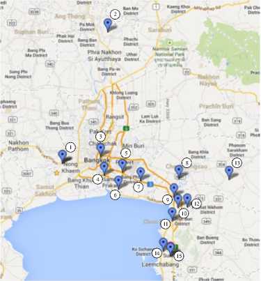
Fig 2. Destination locations of the BN region

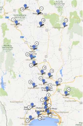
Fig 3. Destination locations of the CT region

Fig 1. Pseudocode of the ACS algorithm parts onto more three main regions, i.e. central, northern and northeastern areas. Therefore, four real-world TTP problems of that car factory, i.e. Bangkok and nearby (BN), Central (CT), Northern (NT) and Northeastern (NET) regions, are conducted in this work. Details of the selected TTP problems are briefly described as follows.

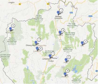
Fig 4. Destination locations of the NT region

For the first TTP problem, the BN region consists of 15

destinations observed by the Google maps [22,23] as shown in Fig. 2. The CT region, the second TTP problem, consists of 22 destinations as virtualized in Fig. 3. The third TTP problem is the NT region consisting of 9 destinations as shown in Fig. 4. Finally, the fourth TTP problem is the NET region consisting of 20 destinations as depicted in Fig. 5.

In order to deliver auto parts, Sammitr has several types of vehicle, i.e. 4-wheel (or pick-up), 6-wheel and 10-wheel tracks. However, among them the 10-wheel truck consumes highest oil fuel. Therefore, the 10-wheel truck is considered in this work. For all selected regions of transportation via 10-wheel truck, Sammitr has to send parts once a week, 4 weeks per month and 12 months per year. For the main energy, the 10-wheel truck consumes one liter of oil fuel for every 4 kilometer (4.0 km/l.). Therefore, the main energy yearly used for transportation (W) in (6) can be rewritten as stated in (7), where E' = 4.0 and T = 4×12.

J x (4 x 12) E

The real distant data in kilometer unit between both destinations of all TTP problems are collected from Google maps [22, 23]. The total distance performed as the objective function ( J ) stated in (1) will be minimized by GA, TS, CS and ACS according to the constraints expressed in (2) – (5), respectively.

Table 1: GA-Parameter Setting for TTP Problems

Entry	TTP	Parameter Settings
	problems	MaxGen	PopN	CrossRate	MutRate

1.	BN	1,000	100	70%	10%
2.	CT	1,000	100	70%	10%
3.	NT	1,000	100	70%	10%
4.	NET	1,000	100	70%	10%

Notes : MaxGen = maximum generation, PopN = number of populations, CrossRate = percentage of crossover and

MutRate = percentage of mutation

Table 2: TS-Parameter Setting for TTP Problems

Entry	TTP problems	Parameter Settings
Entry	TTP problems	MaxCount	R	n	AR
1.	BN	1,000	20%	100	if ( MaxCount = 500) ^ ( R = 10%) if ( MaxCount = 750) ^ ( R = 5%)
2.	CT	1,000	20%	100	if ( MaxCount = 500) ^ ( R = 10%) if ( MaxCount = 750) ^ ( R = 5%)
3.	NT	1,000	20%	100	if ( MaxCount = 500) ^ ( R = 10%) if ( MaxCount = 750) ^ ( R = 5%)
4.	NET	1,000	20%	100	if ( MaxCount = 500) ^ ( R = 10%) if ( MaxCount = 750) ^ ( R = 5%)

Notes : MaxConut = maximum iteration, R = initial search radius, n = number of neighborhood members and AR = adaptive search radius mechanism

Table 3: CS-Parameter Setting for TTP Problems

Entry	TTP problems	Parameter Settings
Entry	TTP problems	MaxCount	R	N	n
1.	BN	1,000	20%	10	100
2.	CT	1,000	20%	10	100
3.	NT	1,000	20%	10	100
4.	NET	1,000	20%	10	100

Notes : MaxConut = maximum iteration for each search direction, R = initial search radius, N = number of search directions and n = number of neighborhood members

Table 4: ACS-Parameter Setting for TTP Problems

Entry TTP problems Parameter Settings MaxCount R N n Radj 1. BN 1,000 20% 10 100 if (MaxCount = 500) ^ (R = 10%) if (MaxCount = 750) ^ (R = 5%) 2. CT 1,000 20% 10 100 if (MaxCount = 500) ^ (R = 10%) if (MaxCount = 750) ^ (R = 5%) 3. NT 1,000 20% 10 100 if (MaxCount = 500) ^ (R = 10%) if (MaxCount = 750) ^ (R = 5%) 4. NET 1,000 20% 10 100 if (MaxCount = 500) ^ (R = 10%) if (MaxCount = 750) ^ (R = 5%)

Notes : MaxConut = maximum iteration for each search direction, R = initial search radius,

N = number of search directions, n = number of neighborhood members and Radj = search radius adjustment

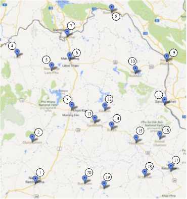
Fig 5. Destination locations of the NET region

for CS, respectively. Algorithms of TS, CS and ACS are coded by MATLAB program, while GA is used from the MATLAB-GA Toolbox [24]. All algorithms will be run on the same platform: Intel Core2 Duo 2.0 GHz 3 GB DDR-RAM computer. Each algorithm performs search on each problem for 100 trials beginning with different initial solutions to obtain the best solution. For a fair comparison, search parameters of GA, TS, CS and ACS are priori set and summarized in Table 1 – Table 4, respectively, in which MaxGen of GA and MaxCount of TS, CS and ACS are used as the termination criteria (TC). The boundaries of destinations are set as the corresponding search spaces.

V. Results and Discussions

After the search stopped, the obtained results over 100 trials running on the same platform are averagely divided

In this paper, algorithms of GA, TS and CS are omitted. Readers may refer to [12] for GA, [11] for TS and [19, 20]

Table 5: Solution Found (Total Distance) of TTP Problems

Entry	TTP problems	Solutions and Methods
Entry	TTP problems	Solutions (km.)	GA	TS	CS	ACS
1.	BN	Min	572	572	572	572
		Max	581	581	581	573
		Mean	574.24	572.74	572.31	572.03
		Std.	2.97	2.30	1.55	0.17
2.	CT	Min	1,486	1,486	1,486	1,486
		Max	1,525	1,525	1,525	1,525
		Mean	1,520.31	1,500.01	1,488.32	1,487.18
		Std.	12.74	18.81	9.31	6.69
3.	NT	Min	1,340	1,340	1,340	1,340
		Max	1,380	1,380	1,380	1,341
		Mean	1,370.62	1,348.29	1,342.13	1,340.13
		Std.	16.81	15.41	8.74	0.22
4.	NET	Min	1,979	1,979	1,979	1,979
		Max	2,004	2,004	2,004	2,004
		Mean	2,002.49	1,989.82	1,982.27	1,979.81
		Std.	5.97	12.44	8.45	4.29

Notes : Min = minimum value of solution found, Max = maximum value of solution found,

Mean = average value of solution found and Std. = standard deviation of solution found

Table 6: Search Time of TTP Problems

Entry	TTP problems	Search times and Methods
Entry	TTP problems	Times (sec.)	GA	TS	CS	ACS
1.	BN	Min	42.05	29.14	18.68	7.78
		Max	74.00	51.96	33.58	15.77
		Mean	59.33	39.27	26.35	11.64
		Std.	9.48	6.54	4.59	2.20
2.	CT	Min	54.05	34.42	13.56	7.87
		Max	100.27	73.08	31.42	17.79
		Mean	78.38	55.85	22.50	12.82
		Std.	13.92	10.16	4.71	2.72
3.	NT	Min	42.93	31.24	22.87	13.80
		Max	73.78	52.17	40.79	23.71
		Mean	57.19	41.17	31.83	18.51
		Std.	8.45	6.40	5.25	2.83
4.	NET	Min	59.56	42.10	28.42	14.79
		Max	96.88	68.00	46.35	26.72
		Mean	78.89	54.95	37.09	20.95
		Std.	11.16	7.84	5.25	3.54

Notes : Min = minimum value of search time, Max = maximum value of search time,

Mean = average value of search time and Std. = standard deviation of search time into two groups, i.e. the quality of the solution (total distance) found as summarized in Table 5 and the search time consumed as provided in Table 6. As average results of solution quality in Table 5, it was found that for all TTP problems the ACS provides better solution than GA, TS and CS. The CS provides better solution than GA and TS. The TS provides better solution than GA, respectively. As average results of search time in Table 6, the search time consumed by the ACS is 23.78% of that consumed by the GA, 33.92% of that consumed by the TS and 53.95% of that consumed by the CS, respectively. This means that the ACS can save the search time of 76.22% when compared with the GA, 66.08% when compared with the TS and 46.06% when compared with the CS. It was found that the ACS averagely spends less search time than others for all problems. However, the best results (shortest distance) of all TTP problems found by GA, TS, CS and ACS are the same values (see Table 5). This can be averagely concluded that the ACS outperforms other algorithms and provides solutions with the best quality within the shortest search time. Details of solution found are discussed as follows.

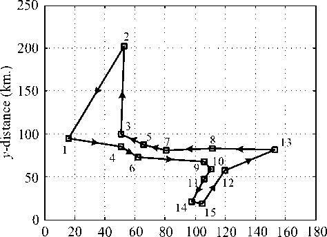
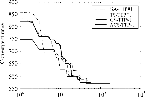
The best solutions of the BN region found by GA, TS, CS and ACS are collected in Table 7 and depicted in Fig. 6 with their corresponding convergent rates shown in Fig. 7. To compare the real route, the best sequence of destination is implemented by Google maps as virtualized in Fig. 8. As the best results of BN region in Table 7 and Fig. 6, it was found that the total distances obtained by the GA, TS, CS and ACS are equal to 572 km., while that obtained by Google maps is equal to 590 km. This means that the best solution found is very satisfactory with the distant error of 3.05%. Occurred error may be due to many possible routes in BN region. In addition, the straight lines in Fig. 6 connecting between dual destinations only represent the sequence of destination. They do not stand for the real distance between such the destinations.

x -distance (km.)

Fig 6. Best direction for BN region by GA, TS, CS and ACS

Table 7: Best Solution for BN Region by GA, TS, CS and ACS

Methods	Solutions (sequence of destination)	Total Distance (km.)	Search Time (sec.)
GA	1 → 4 → 6 → 9 → 10 → 11 → 14 → 15 → 12 → 13 → 8 → 7 → 5 → 3 → 2 → 1	572	42.05
TS	1 → 4 → 6 → 9 → 10 → 11 → 14 → 15 → 12 → 13 → 8 → 7 → 5 → 3 → 2 → 1	572	29.14
CS	1 → 4 → 6 → 9 → 10 → 11 → 14 → 15 → 12 → 13 → 8 → 7 → 5 → 3 → 2 → 1	572	18.68
ACS	1 → 4 → 6 → 9 → 10 → 11 → 14 → 15 → 12 → 13 → 8 → 7 → 5 → 3 → 2 → 1	572	7.78

Iterations

Fig 7. Convergent rates of BN region by GA, TS, CS and ACS

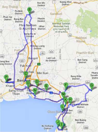
Figure 8. Best sequence of destination of BN implemented by Google maps

The best solutions of the CT region found by GA, TS, CS and ACS are collected in Table 8 and depicted in Fig. 9 with their corresponding convergent rates shown in Fig. 10. To compare the real route, the best sequence of destination is implemented by Google maps as virtualized in Fig. 11. As the best results of CT region in Fig. 9 and Table 8, It was found that the total distance obtained by the GA, TS, CS and ACS is equal to 1,486 km., while that obtained by Google maps is equal to 1,475 km. This means that the best solution found is very satisfactory with the distant error of 0.75%. The error occurred may be due to many possible routes in CT region.

Table 8: Best Solution for CT Region by GA, TS, CS and ACS

Methods	Solutions (sequence of destination)	Total Distance (km.)	Search Time (sec.)
GA	1 → 7 → 8 → 4 → 17 → 12 → 10 → 11 → 19 → 2 → 6 → 22 → 3 → 18 → 13 → 21 → 9 → 20 → 5 → 15 → 16 → 14 → 1	1,486	54.05
TS	1 → 7 → 8 → 4 → 17 → 12 → 10 → 11 → 19 → 2 → 6 → 22 → 3 → 18 → 13 → 21 → 9 → 20 → 5 → 15 → 16 → 14 → 1	1,486	34.42
CS	1 → 7 → 8 → 4 → 17 → 12 → 10 → 11 → 19 → 2 → 6 → 22 → 3 → 18 → 13 → 21 → 9 → 20 → 5 → 15 → 16 → 14 → 1	1,486	13.56
ACS	1 → 7 → 8 → 4 → 17 → 12 → 10 → 11 → 19 → 2 → 6 → 22 → 3 → 18 → 13 → 21 → 9 → 20 → 5 → 15 → 16 → 14 → 1	1,486	7.87

0 50 100 150 200 250 300

x -distance (km.)

Fig 9. Best direction for CT region by GA, TS, CS and ACS

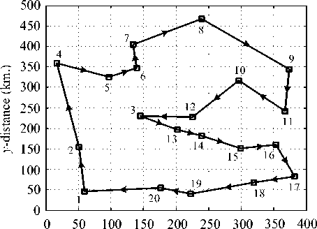
The best solutions of the NT region found by GA, TS, CS and ACS are collected in Table 9 and depicted in Fig. 12 with their corresponding convergent rates shown in Fig. 13. To compare the real route, the best sequence of destination is implemented by Google maps as virtualized in Fig. 14. As the best results of NT region in Fig. 12 and Table 9, it was found that the total distance obtained by the GA, TS, CS and ACS is equal to 1,340 km., while that obtained by Google maps is equal to 1,337 km. This means that the best solution found is very satisfactory with the distant error of 0.22%. The error occurred may be due to many possible routes in NT region.

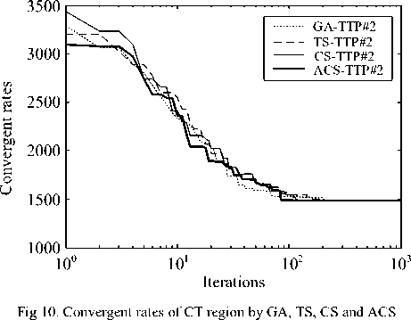
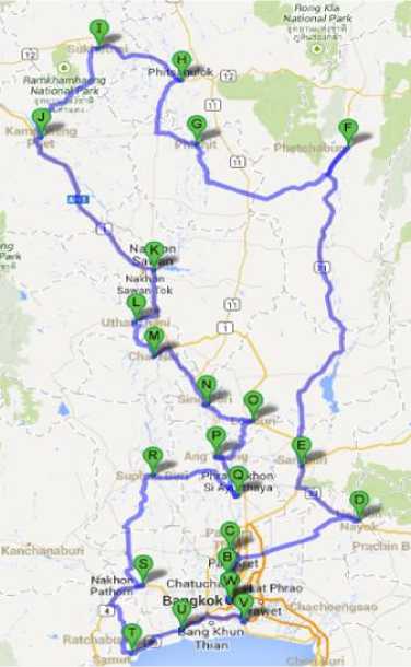
Fig 11. Best sequence of destination of CT implemented by Google maps

Table 9: Best Solution for NT Region by GA, TS, CS and ACS

Methods	Solutions (sequence of destination)	Total Distance (km.)	Search Time (sec.)
GA	1 → 4 → 3 → 5 → 9 → 7 → 8 → 2 → 6 → 1	1,340	42.93
TS	1 → 4 → 3 → 5 → 9 → 7 → 8 → 2 → 6 → 1	1,340	31.24
CS	1 → 4 → 3 → 5 → 9 → 7 → 8 → 2 → 6 → 1	1,340	22.87
ACS	1 → 4 → 3 → 5 → 9 → 7 → 8 → 2 → 6 → 1	1,340	13.80

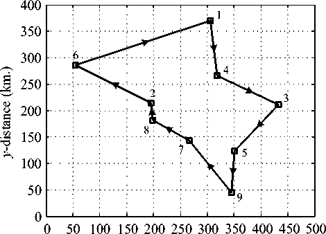
x -distance (km.)

Fig 12. Best direction for NT region by GA, TS, CS and ACS

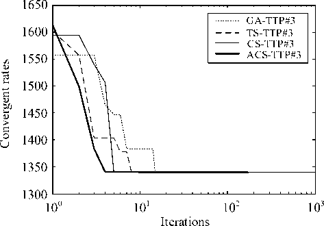
Fig 13. Convergent rates of NT region by GA, TS, CS and ACS

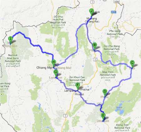
Figure 14. Best sequence of destination of NT implemented byGoogle maps

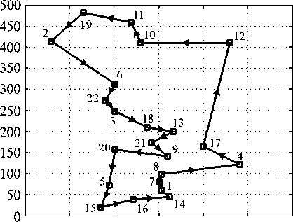
Finally, the best solutions of the NET region found by GA, TS, CS and ACS are collected in Table 10 and depicted in Fig. 15 with their corresponding convergent rates shown in Fig. 16. To compare the real route, the best sequence of destination is implemented by Google maps as virtualized in Fig. 17. As the best results of NT region in Fig. 15 and Table 10, it was found that the total distance obtained by the GA, TS, CS and ACS is equal to 1,979 km., while that obtained by Google maps is equal to 1,979 km. This means that the best solution found is very satisfactory with the distant error of 0.00%.

Table 10: Best Solution for NET Region by GA, TS, CS and ACS

Methods	Solutions (sequence of destination)	Total Distance (km.)	Search Time (sec.)
GA	1 → 2 → 4 → 5 → 6 → 7 → 8 → 9 → 11 → 10 → 12 → 3 → 13 → 14 → 15 → 16 → 17 → 18 → 19 → 20 → 1	1,979	59.56
TS	1 → 2 → 4 → 5 → 6 → 7 → 8 → 9 → 11 → 10 → 12 → 3 → 13 → 14 → 15 → 16 → 17 → 18 → 19 → 20 → 1	1,979	42.10
CS	1 → 2 → 4 → 5 → 6 → 7 → 8 → 9 → 11 → 10 → 12 → 3 → 13 → 14 → 15 → 16 → 17 → 18 → 19 → 20 → 1	1,979	28.42
ACS	1 → 2 → 4 → 5 → 6 → 7 → 8 → 9 → 11 → 10 → 12 → 3 → 13 → 14 → 15 → 16 → 17 → 18 → 19 → 20 → 1	1,979	14.79

x -distance (km.)

Fig 15. Best direction for NET region by GA, TS, CS and ACS

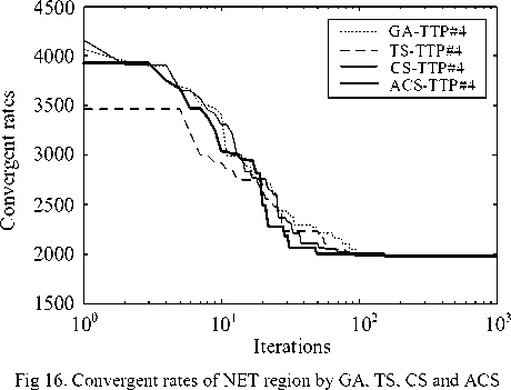
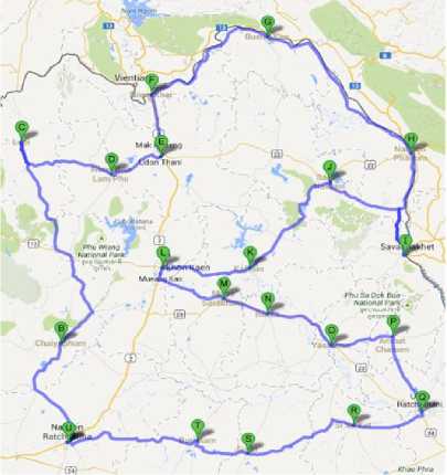
Figure 17. Best sequence of destination of NET implemented by Google maps

To confirm this conclusion for TTP problems, one-way ANOVA statistical method is conducted to compare these results. In order to analyze the results whether there is significance between the results of each algorithm, F-test in the SPSS program is conducted. The hypothesis of this test is expressed in (8) – (9) by using the α = 0.05 (the confidential level of 95%), where H0 is a null hypothesis, H1 is an alternative hypothesis, µ1 is the mean value (of solutions found or search time consumed) of GA, µ2 is the mean value (of solutions found or search time consumed) of TS, µ3 is the mean value (of solutions found or search time consumed) of CS and µ4 is the mean value (of solutions found or search time consumed) of ACS. Comparison results are summarized in Table 11 – Table 14.

H ₀ : µ ₁ = µ ₂ = µ ₃ = µ ₄ (8)

H ₁ : µ _i ≠ µ _j , i ≠ j at least one pair of algorithms (9)

As results of solution quality in Table 11 – Table 12, it was found that for all algorithms, there is significant difference ( p -value < 0.05) among those algorithms. ACS outperforms GA on all four TTP problems (BN, CT, NT and NET), TS on three TTP problems (CT, NT and NET) and CS on one TTP problem (NET). TS, CS and ACS show equal performance on one TTP problem (BN). CS and ACS show equal performance on two TTP problems (CT and NT). This can be noticed that in overall results the ACS has better performance in terms of the quality of solution found. For the results of search time consumed in Table 13 – Table 14, it was shown that for all algorithms, there is significant difference ( p -value < 0.05) among those algorithms. In sense of search time, ACS outperforms GA, TS and CS on all three TTP problems. This can be concluded that in overall results the ACS performs better performance in terms of the search time consumed.

Table 11: One-Way ANOVA of Solution Qualities of TTP Problems

Entry	TTP Problem	Average Optimal Solutions and Standard Deviation				F		p
Entry	TTP Problem	Solutions	GA	TS	CS	ACS
1.	BN	Mean Std.	574.24 2.97	572.74 2.30	572.31 1.55	572.03 0.17	23.426**	.000
2.	CT	Mean Std.	1,520.32 12.74	1,500.04 18.81	1,488.34 9.31	1,487.17 6.69	146.022**	.000
3.	NT	Mean Std.	1,370.60 16.81	1,348.35 15.41	1,342.11 8.74	1,340.05 0.22	131.431**	.000
4.	NET	Mean Std.	2,002.50 5.97	1,989.75 12.44	1,982.25 8.45	1,979.75 4.29	146.029**	.000

Notes: Mean = average value of solution found, Std. = standard deviation of solution found, F = F–value of the F–test, p = p–value, ** = significance results at confidential level of 99%.

Table 12: Significant Comparison of Solution Qualities of TTP Problems

Function Name	Mean Difference of Optimal Solution (I-J)
Function Name	Algorithms	GA TS	CS	ACS
BN	GA	- 1.50**	1.93**	2.21**
	TS	-	0.43	0.71
	CS		-	0.28
	ACS			-
CT	GA	- 20.28**	31.98**	33.15**
	TS	-	11.70**	12.87**
	CS		-	1.10
	ACS			-
NT	GA	- 22.25**	28.49**	30.55**
	TS	-	6.24**	8.30**
	CS		-	2.06
	ACS			-
NET	GA	- 12.75**	20.25**	22.75**
	TS	-	7.50**	10.00**
	CS		-	2.50**
	ACS			-

Table 13: One-Way ANOVA of Search Times of TTP Problems

Entry	Function Average Search Times and Standard Deviation F p Name Times (sec.) GA TS CS ACS
1.	BN Mean 59.33 39.27 26.35 11.64 1,032.41** .000 Std. 9.48 6.54 4.59 2.20
2.	CT Mean 13.92 10.16 4.71 2.72 1,121.20** .000 Std. 1.39 1.02 0.47 0.27
3.	NT Mean 57.19 41.17 31.83 18.51 715.50** .000 Std. 8.45 6.40 5.25 2.83
4.	NET Mean 78.89 54.95 37.09 20.95 1,092.75** .000 Std. 59.33 39.27 26.35 11.64 Table 14: Significant Comparison of Search Times of TTP Problems

Function Mean Difference of Search Time (I-J)

Name	Algorithms GA TS CS ACS
BN	GA - 20.06 32.98 47.69 TS - 12.92 27.63 CS - 14.71 ACS -
CT	GA - 22.54 55.88 65.56 TS - 33.35 43.03 CS - 9.68 ACS -
NT	GA - 16.02 25.36 38.68 TS - 9.34 22.66 CS - 13.32 ACS -
NET	GA - 23.94 41.80 57.94 TS - 17.86 34.00 CS - 14.71 ACS -

Referring to results of all four TTP problems in Table 5, the best results (shortest distance) of all problems can be found by GA, TS, CS and ACS with the same values. In energy resource management context, the main energy (oil fuel for 10-wheel truck) used for transportation can be yearly calculated by (7). Percent of decreased energy per year ( PDE ) can be calculated by (10), where W lowest is total energy per year obtained by the lowest-performance method and W_higher is total energy per year obtained by the higher-performance methods. The best results providing the optimal energy consumed are summarized in Table 15. It was found in Table 15 that the optimal energy for all TTP problems can be achieved by GA, TS, CS and ACS. However, the ACS can provide the optimal solution faster than others.

PDE = 100 xf W lowest - W higher ) (10) V W lowest J

Once the average results of all four TTP problems in Table 5 is considered, the average results (averagely shortest distance) of all TTP problems found by GA, TS, CS and ACS are different. In energy resource management context, the main energy used can be yearly calculated by (7) and also PDE can be calculated by (10). The best results providing the optimal energy consumed are summarized in Table 16. It was found in Table 16 that for the first TTP (BN) problem once compared with GA which is the lowest-performance method, the PDE of

0.26%, 0.34% and 0.38% can be decreased by TS, CS and ACS, respectively. For the second TTP (CT) problem once compared with GA, the PDE of 1.34%, 2.10% and 2.18% can be decreased by TS, CS and ACS, respectively. For the third TTP (NT) problem once compared with GA, the PDE of 1.63%, 2.08% and 2.22% can be decreased by TS, CS and ACS, respectively. Finally for the fourth TTP (NET) problem once compared with GA, the PDE of 0.63%, 1.01% and 1.13% can be decreased by TS, CS and ACS, respectively. Although these results are not quite significant, the maximum percent of decreased energy per year of all TTP problems can be successfully achieved by the ACS. Moreover, the ACS still provide the averagely optimal solution faster than other candidate algorithms.

VI. Conclusions

Optimization of real-world traveling transportation problems (TTP) of a specific car factory by the adaptive current search (ACS) metaheuristics according to energy resource management optimization context has been proposed in this paper. The total distance of the selected TTP has been performed as the objective function to be minimized to decrease the energy consumption. Four real-world TTP problems of a selected factory in Thailand, i.e. Bangkok and nearby (BN), Central (CT), Northern (NT) and Northeastern (NET) regions, are conducted. As results by comparison with the genetic

Table 15: Best Results of Energy Resource Management of TTP Problems

Entry1: BN region
Methods	Total distance (km.)/issue	10-Wheel’s Oil fuel (l.)/issue	Total distance (km.)/year	10-Wheel’s Oil fuel (l.)/year	PDE (%)	Search time (sec.)
GA	572	143	27,456	6,864	0.00	42.05
TS	572	143	27,456	6,864	0.00	29.14
CS	572	143	27,456	6,864	0.00	18.68
ACS	572	143	27,456	6,864	0.00	7.78
Entry2: CT region
Methods	Total distance	10-Wheel’s	Total	10-Wheel’s	PDE	Search time
	(km.)/issue	Oil fuel (l.)/issue	distance (km.)/year	Oil fuel (l.)/year	(%)	(sec.)
GA	1,486	371.50	71,328	17,832	0.00	54.05
TS	1,486	371.50	71,328	17,832	0.00	34.42
CS	1,486	371.50	71,328	17,832	0.00	13.56
ACS	1,486	371.50	71,328	17,832	0.00	7.87
Entry3: NT region
Methods	Total distance	10-Wheel’s	Total	10-Wheel’s	PDE	Search time
	(km.)/issue	Oil fuel (l.)/issue	distance (km.)/year	Oil fuel (l.)/year	(%)	(sec.)
GA	1,340	335	64,320	16,080	0.00	42.93
TS	1,340	335	64,320	16,080	0.00	31.24
CS	1,340	335	64,320	16,080	0.00	22.87
ACS	1,340	335	64,320	16,080	0.00	13.80
Entry4: NET region
Methods	Total distance	10-Wheel’s	Total	10-Wheel’s	PDE	Search time
	(km.)/issue	Oil fuel (l.)/issue	distance (km.)/year	Oil fuel (l.)/year	(%)	(sec.)
GA	1,979	494.75	94,992	23,748	0.00	59.56
TS	1,979	494.75	94,992	23,748	0.00	42.10
CS	1,979	494.75	94,992	23,748	0.00	28.42
ACS	1,979	494.75	94,992	23,748	0.00	14.79

Table 16: Average Results of Energy Resource Management of TTP Problems

Entry1: BN region Methods Total distance (km.)/issue 10-Wheel’s Oil fuel (l.)/issue Total distance (km.)/year 10-Wheel’s Oil fuel (l.)/year PDE (%) Search time (sec.) GA 574.24 143.56 27,563.52 6,890.88 - 59.33 TS 572.74 143.19 27,491.52 6,872.88 0.26 39.27 CS 572.31 143.08 27,470.88 6,867.72 0.34 26.35 ACS 572.03 143.01 27,457.44 6,864.36 0.38 11.64 Entry2: CT region Methods Total distance 10-Wheel’s Total 10-Wheel’s PDE Search time (km.)/issue Oil fuel (l.)/issue distance (km.)/year Oil fuel (l.)/year (%) (sec.) GA 1,520.31 380.08 72,974.88 18,243.72 - 78.38 TS 1,500.01 375.00 72,000.48 18,000.12 1.34 55.85 CS 1,488.32 375.08 71,439.36 17,859.84 2.10 22.50 ACS 1,487.18 371.80 71,384.64 17,846.16 2.18 12.82 Entry3: NT region Methods Total distance 10-Wheel’s Total 10-Wheel’s PDE Search time (km.)/issue Oil fuel (l.)/issue distance (km.)/year Oil fuel (l.)/year (%) (sec.) GA 1,370.62 342.66 65,789.76 16,447.44 - 57.19 TS 1,348.29 337.07 64,717.92 16,179.48 1.63 41.17 CS 1,342.13 335.53 64,422.24 16,105.56 2.08 31.83 ACS 1,340.13 335.03 64,326.24 16,081.56 2.22 18.51 Entry4: NET region Methods Total distance 10-Wheel’s Total 10-Wheel’s PDE Search time (km.)/issue Oil fuel (l.)/issue distance (km.)/year Oil fuel (l.)/year (%) (sec.) GA 2,002.49 500.62 96,119.52 24,029.88 - 78.89 TS 1,989.82 497.46 95,511.36 23,877.84 0.63 54.95 CS 1,982.27 495.57 95,148.96 23,787.24 1.01 37.09 ACS 1,979.81 494.95 95,030.88 23,757.72 1.13 20.95 algorithm (GA), tabu search (TS) and current search (CS), it was found that the ACS outperforms other algorithms and could provide very satisfactory solutions within faster search time. Once compared with the practical data implemented by Google maps, there exists distant error of no longer than 3.05% form the results obtained by the ACS. The maximum percent of decreased energy per year of all TTP problems can be successfully achieved by the ACS. This can be concluded that the performance of the ACS is superior to that of GA, TS and CS to optimize the TTP problems. For the future research, the ACS will be applied to other more complicate forms of TTP problem including the multivehicle and traffic jam factor and so forth to gain more effectiveness of the ACS.

Acknowledgement

The authors wish to thank Sammitr Motors Manufacturing Public Co., Ltd., Samut Sakhon, Thailand for supporting the practical data of TTP problems. Sincere thanks are due to the editor and anonymous reviewers for their constructive comments.

Список литературы Traveling Transportation Problem Optimization by Adaptive Current Search Method

S. Kikuchi and P. Chakroborty, Place of possibility theory in transportation analysis, Transportation Research, Part B, vol.40, pp.595-615, 2006.
G. Reinelt, The Traveling Salesman: Computational Solutions for TSP Applications. Springer-Verlag, 1994.
M. Bellmore and G. L. Nemhauser, “The traveling salesman problem: a survey,” Operation Research, vol.16, 1986, pp.538-558.
E. L. Lawler, J. K. Lenstra, A. H. G. Rinnooy Kan and D. B. Shmoys, The Traveling Salesman Problem: A Guided Tour of Combinatorial Optimization, John-Wiley & Sons, 1986.
M. Held and R. Karp, “A dynamic programming approach to sequencing problems,” SIAM J, vol.1, 1962, pp.196-210.
J. Little, K. Murty, D. Sweeney and C. Karel, “An algorithm for the traveling salesman problem,” Operation Research, vol.12, 1963, pp.972-989.
M. Padberg and G. Rinaldi G, “A branch-and-cut algorithm for the resolution of large-scale traveling salesman problem,” SIAM Review, vol.33, 1991, pp.60-100.
G. B. Dantzig, D. R. Fulkerson, and S. M. Johnson, “Solution of a large scale traveling salesman problem,” Operation Research, vol.2, 1954, pp.393-410.
E. H. L. Aarts, J. H. M. Korst and P. J. M. Laarhoven, “A quantitative analysis of the simulated annealing algorithm: a case study for the traveling salesman problem,” J. of Stats Phys, vol. 50, 1988, pp.189-206.
J. V. Potvin, “The traveling salesman problem: a neural network perspective,” INFORMS J. of Computing, vol. 5, 1993, pp. 328-348.
C. N. Fiechter, “A parallel tabu search algorithm for large scale traveling salesman problems,” Discrete Applied Mathematics, vol. 51(3), 1994, pp. 243-267.
J. V. Potvin, “Genetic algorithms for the traveling salesman problem,” Annuals of Operation Research, vol.63, 1996, pp.339-370.
Y.-H. Liu, “A hybrid scatter search for the probabilistic traveling salesman problem,” Computers & Operations Research, vol.34, 2007, pp.2949-2963.
X. C. Shi, Y. C. Liang, H. P. Lee, C. Lu and Q. X. Wang, “Particle swarm optimization-based algorithms for TSP and generalized TSP,” Information Processing Letters, vol.103, 2007, pp.169-176.
B. Bontoux and D. Feillet, “Ant colony optimization for the traveling purchaser problem,” Computers & Operations Research, vol.35, 2008, pp.628-637.
S. Suwannarongsri and D. Puangdownreong, “Adaptive tabu search for traveling salesman problems,” International Journal of Mathematics and Computers in Simulation, iss.2, vol.6, 2012, pp.274-281.
S. Suwannarongsri, T. Bunnag and W. Klinbun, “Energy resource management of assembly line balancing problem using modified current search method,” International Journal of Intelligent Systems and Applications, vol.6, no.3, 2014, pp.1- 11.
S. Suwannarongsri, T. Bunnag and W. Klinbun, “Optimization of energy resource management for assembly line balancing using adaptive current search,” American Journal of Operations Research, vol.4, no.1, 2014, pp.8-21.
A. Sukulin and D. Puangdownreong, “A novel meta-heuristic optimization algorithm: current search,” Proceeding of the 11th WSEAS International Conference on Artificial Intelligence, Knowledge Engineering and Data Bases (AIKED '12), 2012, pp.125-130.
A. Sukulin and D. Puangdownreong, “Control synthesis for unstable systems via current search,” Proceeding of the 11th WSEAS International Conference on Artificial Intelligence, Knowledge Engineering and Data Bases (AIKED '12), 2012, pp.131-136.
Sammitr Motors Manufacturing Public Co., Ltd., 2013. http://www.sammitr.com.
A. C. Madrigal, “How google builds its maps-and what it means for the future of everything,” The Atlantic, 6 September, 2012, retrieved on 9 February 2013.
B. Liebert, “Create, collaborate and share advanced custom maps with google maps engine lite (Beta),” Google Maps. Google, Inc., retrieved on 20 May 2013.
MathWorks, Genetic Algorithm and Direct Search Tool-box: For Use with MATLAB. User’s Guide, vol.1, MathWorks, Natick, Mass, 2005.

Еще

Статья научная