Tree-serial parametric dynamic programming with flexible prior model for image denoising

A low-level processing is an important preliminary step in almost every image analysis system. Images may be corrupted by a disruptive noise during acquisition and transmission process. Thus, one of the main objectives of this low-level processing is to suppress noise, taking into account the essential requirement to preserve the local image structure for accurate and efficient subsequent analysis.The practical importance of noise suppression for image processing and computer vision keeps up a constant attention from the scientists. Many methods for edgepreserving image denoising [1 – 7] have been proposed in the literature, but none of them can simultaneously achieve both sufficient accuracy to provide a highly reliable data and computational speed to process super-resolution or dynamic images at a practice-relevant time. Therefore, denoising is still a challenging problem.

We apply here Bayesian approach as, perhaps, one of the most conceptually attractive and popular approaches to image processing. In the Bayesian framework, the problem of image denoising can be expressed as the problem of estimation of a hidden Markov component X = ( x t , t ∈ T ), T =( t = { t 1 , t 2 }, t 1 = 1... N 1 , t 2 = 1... N 2 ) of a two-component ( X , Y ) Markov random field (MRF), where the analyzed noisy image Y = ( y t , t ∈ T ) plays the role of the observed component.

In the case of a singular loss function, the Bayesian estimation of the component X can be found as a maximum a posteriori probability (MAP) estimation. It leads to the minimization problem of the objective function of a special kind related to the equivalent representation of Markov random fields in the form of Gibbs random fields in accordance with Hammersley–Clifford Theorem [8]. This function is often called the Gibbs energy function [9] and is formed as a sum of elementary objective functions of one or two variables associated, respectively, with nodes and edges of the pixel neighborhood graph.

The undirected graph that reflects occurring of pairs of variables in the given pairwise separable objective function is called the adjacency graph. Functions of one or two variables represent Gibbs potentials on cliques of adjacency graph and will be called node and edge functions correspondingly.

The edge functions are used to define the prior model of a hidden field X and have a crucial influence on the edge-preserving properties. Different types of prior assumptions result in different types of edge functions. Various non-convex pairwise edge functions are considered in the literature [9-11] for preserving significant differences of values in the corresponding pairs of adjacent elements and smoothing the other differences. Convex edge-preserving pairwise potential functions were proposed to avoid the numerical involutions arising with non-convex regularization. However, non-convex regularization offers the best possible quality of image reconstruction with neat and exact edges [10]. One of the main problems in these approaches is the high computational complexity of corresponding minimization procedures which can hardly be applied to high-resolution images.

In this work, we develop parametric procedures for edge-preserving in image denoising based on dynamic programming (DP) principle, which consists in a recurrent decomposition of the initial problem of minimizing multivariate function into a succession of partial problems, each of which consists in minimizing a function of only one variable. These functions of one variable are called Bellman functions [12].

When the pairwise Gibbs potentials are selected as a minimum of a finite set of quadratic functions, and node functions are in quadratic form, the Bellman functions at each step of the dynamic programming will have a form of a minimum of a finite set of quadratic functions [11, 13, 14]. This lets us keep in memory and recalculate the parameters of these quadratic functions only, instead of using discrete variables and calculation of the DP table, and therefore to reduce the overall computational time.

If the adjacency graph is a tree, then we have a version of a serial dynamic programming procedure [15] namely the tree-serial dynamic programming [16]. For images, the general form of the objective function will be the pairwise separable function with lattice-like adjacency of variables, so the tree-serial DP cannot be applied immediately to the image processing problems.

In our previous works, two different forms of tree-like representation of a rectangular lattice were utilized: treelike approximation by the succession of simple trees [12], and the full set of possible acyclic adjacency graphs [17, 18]. The procedures can effectively remove an additive white Gaussian noise with high quality. Nevertheless, in both methods, the final decision for each variable is made based on a separate graph or the set of graphs. This can lead to inconsistency of the solution with the initial set of prior preferences. To overcome this obstacle, we propose an extended version of a multi quadratic dynamic programming procedure for image denoising based on the partitioning of the initial lattice on the non-overlapping set of chain-like graphs and iterative evaluation of separate groups of goal variables related to these graphs in accordance to the Gauss-Seidel method.

The experimental results show that the method usually converges within five-six iterations and exhibits the clear improvements in the denoising quality. Additionally, we have provided a comparison of the proposed approach with the other procedures for edge-preserving image denoising such asnonlinear total variation (TV) [4], modified Perona– Malik (MP-M) [7], Beltrami [19].

Related work

Within the Bayesian framework, the final decision about the hidden component X = ( x _t , t e T) of a two-component ( X , Y ) MRF is based on posterior probability density distribution. The principle of average risk minimization in combination with singular loss function leads to the wide-spread decision rule, known as maximum a posteriori probability (MAP) estimation [9].

It is important that the pixel grid of an image is naturally supplied by the binary neighborhood relation, which turns it into a graph. The simplest case of such a graph is a rectangular lattice G = ( T×T ) (Fig. 1) which considers pairwise relations only and therefore has the clique number equal to two. In this case, the objective function for MAP estimation in the form of so-called Gibbs energy [9], will be the sum of functions of no more than two variables namely, the node and the edge ones [14]:

J ( X | Y ) \ u t ( x 1 1 Y ) + £ _Y t ‘, t-( x t ‘ , x t-) . (1) t e T ( t ', t ")

In the papers [11, 14] we proposed to use a non-convex type of pairwise potential functions, that allow to flexibly set a priori preferences, using distinctpenalty coefficients for various ranges of differences between the values of adjacent image elements:

Y t - ( x t - , xf ) = u min[ Y ⁽1) ( x t - , xt " ), • •

Y t ^’ 1) ( x t - , x t - ), A 2 ]

,

,

where A , u - smoothing parameters, L - a number of quadratic functions,

Y t‘) ( x _t - , x _t -- ) = X ⁽ i ) ( x _t - - x _t -- ) ² + d ⁽ i ) -quadratic functions with parameters X ⁽i ) и d ⁽ i ) , i = 1,..., L -1, ( t' , t ") e G .

These pairwise potential functions have the desired properties for the conservation of abrupt changes in the analyzed data.

Node functions are chosen in the quadratic form:

V t ( x t ) = ( x t - y t ) ² .

When the pairwise Gibbs potentials are selected as a minimum of a finite set of quadratic functions (2), and node functions are in quadratic form (3), the Bellman functions at each step of the dynamic programming will also be a minimum of a finite set of quadratic functions. Therefore, each Bellman function belongs to the same parametric family, which leads to the parametric procedure called multi quadratic dynamic programming procedure (MQDP) [11, 13, 14].The procedure searches for the minimum of theobjective function (1) in two passes according toforwardand backward recurrent relations [13, 14].

In the case of the graph G is a chain, the forward recurrent relation the Bellman function will be defined [12] in the following way:

Jt (xt) = vt (xt) + min Г Yt (xt-1, xt) + Jt-1 (xt-i)l, (4) xt-1L t = 2,^N, .J1(x1) = V1(x1).

Let F’t (xt) = min pyt (xt-1, xt) + Jt-1(xt-1)!

xt-1 LJ be a partial Bellman function. We have:

Jt ( x t ) = V t ( x_t ) + 7^ ( x t ).

The global minimum of the Bellman function (4) of the last variable min x_N J N ( x N ) coincides with the global minimum of the total objective function for all variables:

xc n = arg min x N J n ( xn ).

The other variables can be found by applying backward recurrent relation [12]:

x t - 1 ( x t ) = arg min ^p y t ( x t - 1 , x t ) + J t - 1 ( x t - 1 ) ] .

^xt - 1

The amount of quadratic functions grows at each step of the forward move but not all of them take part in forming the minimum. These functions can be dropped using simple enough procedure that considers the position of the minimum point and the points of intersection of quadratic functions with each other (Algorithm 1).

It was proven, that in the case of signal processing the number of quadratic functions L_t , that are required for representation of a Bellman function J_t ( x ), generally, is not increased by more than one at each step.

For images, the general form of the objective function will be the pairwise separable function with lattice-like

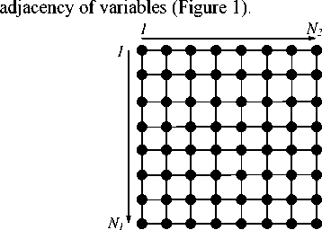
Fig. 1. Neighborhood graph on the set of data array elements: a rectangular lattice n2

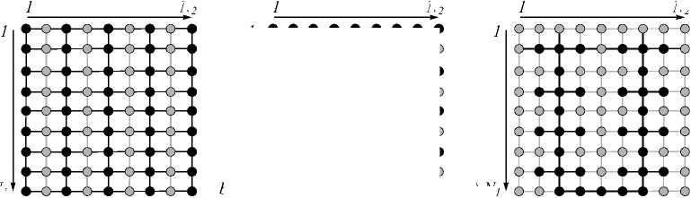
A lattice is not a chain, and Bellman’s DP principle cannot be immediately applied to solving such optimization problems. There are, at least, four ways [16, 17] of using computational advantages of the tree-serial DP for optimization of an objective function with a lattice-like graph of variable adjacency (Figure 2).

The first, and the most often applied to various image processing problems techniqueis based on the following heuristic idea [12]. We can decompose the original lattice-like adjacency graph into several tree-like ones each of which covers, nevertheless, all the elements of the pixel grid. Respectively, instead of the overall objective function, we use several partial functions with tree-like n2

adjacency of variables to evaluate the goal variables at every single row of the original rectangular lattice.

a)

c)

Fig. 2. Examples of the decomposition of a lattice-like adjacency graph into the set of subtrees: (a) odd and even columns, (b) odd and even rows, (c) more complex decomposition into two trees

n2

For this combination of partial pixel neighborhood trees, the algorithm of finding the optimal values of the stem-node variables boils down to a combination of two usual DP procedures, dealing with single, respectively, horizontal and vertical rows of the image.

Hereinafter we will call this procedure the tree approximation algorithm.

We use a separate pixel neighborhood tree, which is defined, nevertheless, on the whole pixel grid and has the same horizontal branches as the others. The resulting image processing procedure is aimed at finding optimal values only for the hidden variables at the stem nodes in each tree. For this combination of partial pixel neighborhood trees, the algorithm of finding the optimal values of the stem-node variables boils down to a combination of two usual dynamic programming procedures, each deal with single, respectively, horizontal and vertical image rows considered as signals on the one-dimensional argument axis [20, 21]. First, such a one-dimensional procedure is applied to the horizontal rows independently for each column to find so-called marginal functions J t ( x t ) which represent the minimum of partial criterion, associated with the particular row with respect to all variables besides x t [22]: ■*■

J t ( X t ) = F t ( X t ) + F t ⁺ ( X t ) + V t ( X t ),                  (6)

where

F t ⁽ x t ) = min [_Y t ⁽ x t — 1 , x t ) + F - 1 ⁽ x t — 1 ) ₊ v t - 1 ⁽ x t - 1 ) ] , x t - 1

and

F t + ( x t ) = min ^[ Y t ( x t , x t + 1 ) + F t + 1 ( X t + 1 ) + V t + 1 ( X t + 1 ) ! .

X t + 1

Then, the procedure is applied to the vertical rows independently for each row with the only alteration: the respective marginal node functions J t ( x t ), obtained at the first step, are taken instead of the image-dependent node functions v t ( Xt ). In the case of real-valued variables x _t and quadratic pairwise separable objective function, these elementary procedures applied to single horizontal and vertical rows are nothing else than Kalman filters-interpolators [23] of a special kind. Nevertheless, using MQDP for processing two-dimensional data based on the tree approximation of lattice-like neighborhood graph, the number of quadratic functions in the Bellman functions may be too large and leads to a lack of effective implementation of the procedure. In paper [11, 14] the following heuristic technique was proposed to preserve the general form of a Bellman function with several minimums. The idea was to divide the quadratic functions into groups. The number of groups is determined by the number of stored minimum values. For the separation of functions into the group, we used the featureless modification of the most popular clustering algorithms – k-means, which possesses the benefits of speed and ease of implementation [14].

In the paper [17] another way for the tree-like approximation of a lattice based on the full set of acyclic adjacency graphs was proposed. Let a hypothetical covering set of all spanning acyclic graphs (the full set) be given. For the finite set of image elements, the number of such graphs is also finite. Let us assume that all elements of the data array be roots for several unknown for us acyclic adjacency graphs from the full set. Expanding step-by-step vicinities of descendants for each element simultaneously, we can obtain its maximal vicinity including the element itself, and thus obtain the final decision for that element as a combination of decisions based on acyclic adjacency graphs from the full set. The paper describes the general probabilistic framework for dependent objects recognition.

The third way [21] consists in finding such a cut of the graph G that it gets resolved into trees G 1 , G 2 , . , G K ; G = J K = 1 GJ, G i ft G j = 0 , i * j . Then, it will be possible to apply the Gauss-Seidel iteration method to optimize the entire objective function by finding, at each step, the global optimum of each of the partial objective functions on trees G ⁱ , i = 1,..., K using tree-serial DP.

Algorithms based on the iterative reevaluation of groups of variables are significantly more robust to local extrema.

The fourth technique considers the lattice as a chain of rows, so, we can consider the variables in each row as an aggregated variable and apply the serial dynamic programming technique which is a particular case of tree-serial dynamic programming [24]. However, the Bellman functions will be functions of as many variables as long are the rows. Nevertheless, the computational complexity of such a procedure will be linear with respect to the number of rows, remaining, though, very high relative to their length. To further reduce the computational complexity of optimization, we heuristically approximate the genuine Bellman functions by appropriate pairwise separable substitutes. However, it is hard to find an appropriate approximation in the case of an edge-preserving Gibbs potentials and we cannot apply this way of approximation in our case.

Approximation algorithms allow constructing the multi quadratic dynamic programming procedures for image processing on the basis of tree-approximation and the full set of adjacency graphs [17, 25]. The second procedure utilizes an increased accuracy of the tree-like representation of a lattice based on the full set of adjacency graphs, described in [18], and let us to sufficiently simplify the recalculation of the intermediate Bellman functions.

Nevertheless, in both methods, the final decision is made based on a separate graph or the set of graphs. This can lead to inconsistency of the solution with the initial set of prior preferences. A construction of an enhanced version of MQDPbased on the partitioning of the initial lattice on the set of non-overlapping set of chain-like graphs and iterative evaluation of separate groups of goal variables related to these graphs in accordance to the Gauss-Seidel method can improve the overall accuracy of image denoising.

Iterative multi-quadratic procedure

As described in the previoussection, we can find such a cut of the graph G that it gets resolved into two trees. Then, it will be possible to apply the Gauss-Seidel iteration method to optimize the entire objective function by finding, at each step, the global optimum of each of the two-partial objective function using tree-serial dynamic programming. One of the simplest ways to divide a lattice graph into trees is to combine all the variables into two groups, namely the variables corresponding to the odd and even rows of the original lattice. Moreover, a chainlike decomposition let us skip the k-means clustering step of reducing the number of quadratic functions in the representations of Bellman functions [11, 14], as the node functions remain in quadratic form at each iteration step. This can greatly reduce the computation complexity of the procedure.

Further, in accordance with the Gauss-Seidel principle, starting from some initial approximation, we carry out optimization with respect to the first group of variables, for fixed values of the variables of the second group. Then we carry out optimization with respect to the variables of the second group, with the fixed values of the first group found in the previous step, etc. until the procedure converges, and the local minimum of the criterion is reached.

As before [11, 14, 18] we will use Algorithm 1 to select quadratic functions in the representation of the Bellman functions at each step of dynamic programming.

Algorithm 1:Reduction of a number of quadratic functions

Input: F t (i ) ( x _t ), i = 1,..., K t _t .

Output: F t i ) ( x _t ), i = 1,..., K t 't , K t 't <  K t _t

• 1.    In the beginning, sort by ascending values d _t ^{( i )} of

• 2.    In case of the presence of a parameter A at each step, we look for the minimum constant D t = d t ⁽¹⁾ + u - A ² and reject all other constants.

• 3.    Discard all functions that have minimum greater than or equal to this constant

• 4.    Among the remaining functions, select the function with the smallest minimum and keep it.

• 5.    Find and check the necessary and sufficient condition of the intersection of quadratic functions by equations. Discard all the functions for which there is no intersection.

• 6.    Among the remaining functions, select the function with the smallest minimum and keep it.

• 7.    Repeat until there exist functions for which no decision on acceptance or discarding is done.

the array F _t ⁽ i ) ( x _t ) .

t ⁽ i ) >  D t , i = 2 . j< t .

The proposed iterative multi-quadratic procedure for image denoising is described in Algorithm 2.

However, the Gauss-Seidel method guarantees to find the global optimum only if the objective function is convex or concave. But the described above procedure can improve the quality of initial approximation obtained by means of noniterative multi quadratic dynamic programming procedure. Thus, the general algorithmic scheme of solving pairwise separable optimization problem consists in two steps. At first, the initial approximation must be found by means of the fast tree approximation algorithm, and then the iterative tree-decomposition procedure starts from this approximate solution.

To overcome the locality effect of the Gauss-Seidel search, the can change the way of decomposition as soon as the next local minimum is achieved. The computational complexity of each iteration is linear relative to the number of pixels.

The initial approximation X * = ( x * , t e T ) could be chosen in different ways. For example, we can start from the observable image itself, or use the results of treedecomposition based procedure [11] or procedure on the full set of adjacency graphs [18] as the initial approximation for faster convergence.

Algorithm 2: Iterative multi-quadratic procedure

Input: Observed image Y = ( y _t , t e T ),

Initial approximation: X * = ( x * t e T ).

MaxIter, oddness = 0.

Output: Resulting image X = ( x _t , t e T ).

• o    while k=1 to MaxIter do

• o    t = t + oddness

o ф t ( x t ) = ( x t - y t ) ² + y ( x t , x * + 1 ) + y ( x t , x * - 1 )

o Calculate functions F _t ( x _t ) by form (5) with node function ф _t ( x _t )and applying Algorithm 1.

• o    Calculate marginal node functions J t ( x t ) with node functions (3) by form (6) and applying Algorithm 1 without his steps 2-3.

o x t ( x _t ) = arg min J _t ( x _t )

• o    t = t + 2

o    (X * ( x * ) = X ( x t ))

• o    oddness=1 – oddness

• o    Return X = ( x _t )

If we apply Algorithm 2 to the rows of the image , then, the t + oddness = { t 1 + oddness , t 2 }, x t –1 means x t ₁–1, t ₂ , and x _{t +1} corresponds to x_{t 1+1, t 2} . In the same time, we can apply Algorithm 2 to the columns of the image, when e.g. the next local minimum is reached. In this case t + oddness = { t 1 , t 2 + oddness }, x t –1 means x t ₁, t ₂–1 , etc.

The previously proposed procedures [11, 14, 18] on the basis of MQDP use different tree-like approximations of the lattice-like pixel grid of an image. Thus, such procedures do not search the minimum of the initial criterion (1). Instead, they form a set of partial criteria that is close in some sense to the initial and find the exact global minimum of this criteria.

In contrast, the procedure described here is intended to solve the initial optimization task but it can provide a local minimum only. Therefore it has different behavior in comparison with the methods [11, 18] and can achieve better results, as evidenced by experiments.

Experimental results

All the experiments were run on a machine with Core i7 – CPU 2GHz, SDRAM 4 GB, Windows 10 (64 bit), and implemented in Matlab.

The test images are 8-bit grayscale standard images with various levels of additive white Gaussian noise. Standard deviations are chosen to be о = 10,20, 30. Denoising results are quantified by the Mean Structure Similarity Index (SSIM) and Peak to Signal Noise Ratio (PSNR) [1].

Details of quantified measurements are shown in Table 1 with different Gaussian noise levels. Results of measurements in Table 1 are averaged over multiple tests.

Table 1. Performance of various methods as measured by PSNR and SSIM corresponding to varying noise levels

Image	House 128×128
о	10	20	30
	PSNN SSIM	PSNR SSIM	PSNR SSIM
TV	28.74 0.8279	26.14 0.7440	24.06 0.6538
M-PM	30.37 0.8559	26.58 0.7337	24.40 0.6499
Beltrami	30.46 0.8695	26.63 0.7544	24.38 0.6679
MQDP	30.48 0.8708	26.60 0.7841	24.30 0.6886
Proposed Horizontal	30.58 0.8801	26.68 0.7949	24.41 0.7418
Proposed Vertical	30.54 0.8798	26.62 0.7930	24.33 0.7397
Proposed Combination	30.68 0.8809	26.72 0.7966	24.43 0.7429
Image	Lake 128×128
TV	25.67 0.8947	23.14 0.8118	20.97 0.7173
M-PM	27.52 0.9183	23.35 0.8192	21.19 0.7359
Beltrami	26.32 0.8997	23.97 0.8438	21.61 0.7660
MQDP	29.54 0.9220	24.09 0.8450	21.27 0.7759
Proposed Horizontal	29.74 0.9268	24.37 0.8591	21.37 0.7923
Proposed Vertical	29.54 0.9250	24.17 0.8564	21.37 0.8003
Proposed Combination	29.84 0.9293	24.52 0.8721	21.79 0.8066
Image	Parrot 128×128
TV	26.06 0.8458	24.30 0.7984	22.76 0.7298
M-PM	29.35 0.9041	25.90 0.7973	23.56 0.7072
Beltrami	28.68 0.8919	25.98 0.8146	23.49 0.7283
MQDP	29.64 0.8955	26.01 0.8380	23.37 0.7376
Proposed Horizontal	29.83 0.9087	26.15 0.8395	23.51 0.7864
Proposed Vertical	29.71 0.8977	26.09 0.8388	23.42 0.7834
Proposed Combination	29.84 0.9177	26.22 0.8411	23.70 0.7886
Image	Hill 256×256
TV	30.30 0.8292	27.78 0.7409	25.97 0.6587
M-PM	30.55 0.8314	27.88 0.7470	25.69 0.6464
Beltrami	30.72 0.8402	28.00 0.7534	25.82 0.6544
MQDP	30.69 0.8579	27.98 0.7610	26.17 0.6842
Proposed Horizontal	30.74 0.8854	28.10 0.7985	26.32 0.7372
Proposed Vertical	30.86 0.8804	28.08 0.7916	26.28 0.7362
Proposed Combination	30.89 0.8865	28.16 0.8055	26.41 0.7381
Image	F16 256×256
TV	30.22 0.8775	26.55 0.7434	24.12 0.6187
M-PM	30.29 0.8845	26.79 0.8005	24.64 0.6425
Beltrami	30.36 0.8896	26.74 0.8244	24.87 0.6815
MQDP	30.50 0.8913	26.88 0.8587	24.75 0.7204
Proposed Horizontal	30.90 0.8927	27.13 0.8688	24.88 0.7334
Proposed Vertical	30.82 0.8921	27.03 0.8668	24.86 0.7387
Proposed Combination	31.04 0.8944	27.18 0.8709	25.03 0.7420
Image	Bridge 256×256
TV	27.40 0.7876	25.63 0.7183	24.16 0.6480
M-PM	29.74 0.8878	26.12 0.7753	24.27 0.6845
Beltrami	30.02 0.8908	26.23 0.7781	24.23 0.6860
MQDP	30.08 0.8982	26.15 0.7898	24.31 0.7079
Proposed Horizontal	30.16 0.9141	26.31 0.8005	24.38 0.7126
Proposed Vertical	30.11 0.9087	26.26 0.7993	24.42 0.7116
Proposed Combination	30.22 0.9159 26.32 0.8028		24.48 0.7140

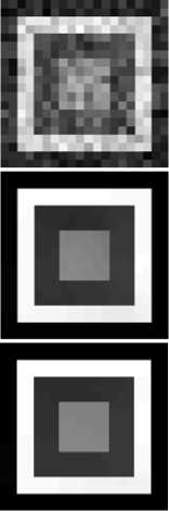
In Fig. 3, we use probe ‘synthetic’ image with the size of 20×20 pixels to compare results of the multi-quadratic procedure (MQDP) [11] and proposed iterative multiquadratic procedure method with iterative horizontal processing, iterative vertical processing, and its combination. A number of iteration steps isequal to 6.

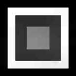
Fig. 3. a) Image “synthetic” with the size of 20×20 pixels;

f )

b)

d)

rion is equal to 2×10 –5 and the maximum number of iterations is set to 2000.

For the M-PM method, the diffusivity parameter is 3, integration constant is set to 0.1 and the number of iterations is the direct proportionality of noise level.

For the TV method, the regularization parameteris set to 0.075, tolerance for convergence criterion is equal to 5×10–4 and the maximum number of iterations is set to 300.

a)

b)

c)

• b)    Noisy PSNR = 18.5907;

• c)    MQDP: PSNR = 29.70, SSIM = 0.9784; d)Iterative horizontal: PSNR = 30.93, SSIM = 0.9862; e) Iterative vertical: PSNR = 31.51, SSIM = 0.9873; f ) Combination: PSNR = 32.94, SSIM = 0.9906

d)

e)

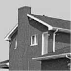
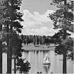
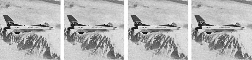
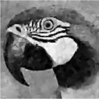
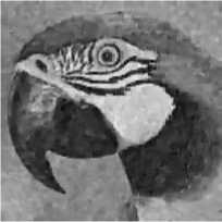
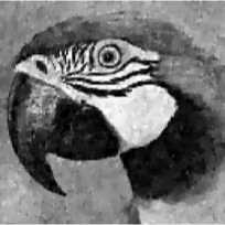
Fig. 4. Original images: a) House, b) Lake, c) Parrot, d) Hill, e) F16, f) Bridge

f)

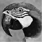
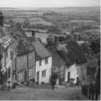
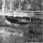
For illustrations, we use the gray level images House, Lake, Parrot, Hill, F16, Bridge. The original images are presented in Figure 4.

Figure 5 and 6 show comparative result images of proposed and other methods for edge-preserving image denoising: Nonlinear Total Variation (TV) [4], Beltrami [19], Modified Perona–Malik (MP-M) [7], Multi quadratic dynamic programming (MQDP) [11].

For Beltrami method, the aspect ratio is set to 1, balancing parameter between fidelity and regularity is the inverse proportionality of noisy level, gradient descent parameter is set to 0.2, tolerance for convergence crite-

For MQDP method, we use edge functions (2) with fixed smoothing parameters values L = 3, λ = 0.2, d = 0.5 Δ ² .

The PSNR and SSIM results for various methods are shown to demonstrate the comparison of their performances.

Conclusion

In this paper, we have tried to discuss promising edge-preserving image denoising methods on the basis of different principles of tree-like representation of an image lattice, and MQDP. A new MQDP version based on the tree-decomposition of the image pixel grid searches for the local minimum for the initial criterion (1), instead of the global minimum of its approximations.

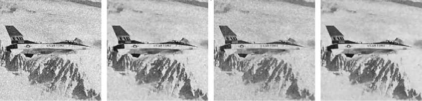
a) Noisy; PSNR= 22.21           b) TV                 c) M-PM               d) Beltrami

e) MQDP               f) Horizontal              g) Vertical             h) Combination

Fig. 5. Results for image “F16” (256×256): Image denoising results of the compared methods

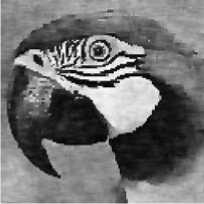
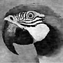
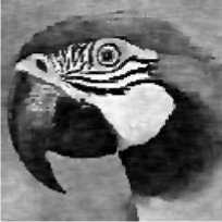
a) Noisy: PSNR = 19.20

b) TV

c) M-PM

d) Beltrami

e) MQDP

f) Horizontal

g) Vertical

h) Combinations

Fig. 6. Results for image “Parrot” (128×128): Image denoising results of the compared methods

The experimental results show that the proposed dynamic programming procedure allows improving the quality of results of multi quadratic dynamic programming. Numerical results show that our proposed algorithms are efficient and allow to obtain result compared or even superior the existed methods.