Turnpike solutions in the problem of excitation transfer along a spin chain

An important class of quantum system control problems is based on the Shr¨odinger equation related to the systems of interacting spins when its Hamiltonian depends linearly on one of controls:

• (1)           Z = — гН(u,u)z,  H = H 0 + diag { h j (t, u) } u,

where z(t) is a complex valued piece-wise smooth N -dimensional vector function, u(t), u(t) are piece-wise continuous real functions, u e R , u e V C R ^p , h j (u) are real continuous functions, H 0 is a constant spin interaction matrix, V is a compact set. System (1) has a dynamic invariant n             n

S = ^ lz ^j (t i ) | 2 = ^ lz ^j (t) | 2 (take S = 1 for definiteness).

j=i            j=i

Quantum systems of such type are associated with investigations in quantum computations ( [1 –4] ). They were investigated numerically in a series of applied works using the Krotov nonlocal iterative method [5] (see, for example [3] ).

Financially supported by the Russian Foundation for Basic Research (pro ject 15-01-01915a, 15-01-01923a).

○c V. I. Gurman⁽ , I. V. Rasina⁽ ,  2016

○c ICS V. A. Trapeznikov of RAS( , 2016

○c Ailamazyan Program System Institute of RAS( ,  2016

○c Program systems: Theory and Applications, 2016

The following optimal control problem is considered. It is given the first spin norm (amplitude) equal to the chain invariant 1 (this implies that initial norms of all the rest spins are equal to zero: z ⁷ (t j ) = 0, j = 1). It is required to transfer the system during the given time to some final state with the least deviation the norm of N -th spin from given value 1:

• (2)    | z 1 (t j ) | = lz } l = 1, J = F (z(t F )) = 1 z ^X (t ! )H inf .

2. Presentation of Original System in Polar Coordinates and Transformations to Derived Systems

In other words it is required to maximize | z ^w (t F ) | , the norm of the final spin at the final time.

Evidently, this finite control problem statement covers the problem of minimal final time t F to reach the state z * (when this functional takes a value of zero), which is important to estimate the quantum speed limit ( QSL ) for the given quantum system. In general, the minimal time problem can be solved correctly as a limit for a sequence of the problems under consideration for different t _Fs < t _{F min} when F(z(t_Fs)) ^ 0. However, in some rather simple cases such as Landau-Zener problem and two-spin chain [6, 7] , it can be solved directly. The following investigations for the approximate solutions and estimates are also carried out in the terms of minimal time transfer.

In [6] it was shown that such problems are degenerate, and it is effective to apply known in the degenerate problems theory basic transformation of the original system to a regular derived system which is especially effective when linear control is unbounded. In [8] this approach was applied to particular cases of the excitation transfer problem [3] for (3 – 5)-spin chains.

This paper is a continuation of [6] . A convenient form of the spin chain as a system of interacted linear oscillators in “polar coordinates” is proposed which is transformed sequentially to derived systems of reducing order up to the first one. Their investigation can be performed analytically or via simple computations, and leads at least to approximate solutions and lower estimates of the transfer time, which can be used in subsequent improving procedures.

We shall consider the following spin-interaction matrix [3]

	— 1    1     0     . ..    0     0 1     — 2    1     . . .    0     0 0    1    — 2  ...   0    0
H o =	...   .. .  .  ...  . .                 .                 .                    ..                 . 0     0     0    ...    — 2    1 ^ 0     0     0    ...    1     —1 )

Then (1) is rewritten as follows

• (3)   z ^j = —г ( (h oj + h j u) z³ + h ij z^{3 1} + h 2j z^{3 +1} ) , j = 1,... ,N,

h oi = h oN = — 1, h ii = h 2N = 0, h iN = h 2i = 1, ^h oj = ^{—2, h} ij = ^h 2j = 1, ^j = 2, .. .^{,N —} 1.

Express every spin as a linear oscillator in “polar coordinates” z ^j = у ³ e ⁴⁰ , y ^j = | z ^j | :

yj = h1jyj-1 sin (0j-i — 0j) + h2jy^+1 sin (0j+1 — 0j), yj > 0, h' = —(h0j + hju) — h1j У—— cos (0j-i — 0j) — h2j У—— cos (0j+1 — 0j).

y ^j                            y ^j

Assume that control variable и is unbounded and coefficients h j are constant, and transform (4) to an equivalent derived system [9, 10] with the use of integrals (y ^j , y ^j ) of the limit system:

dy³/dT = 0, dO³(d-т = —h j , y ^j = 0³ + h j t,   (T = u), 0 ^j = y ^j — h j t,

У ³ = h ij y ^{j 1} sin ((y ^{j 1} — y ^j ) — (h j - i — h j )t )+ ^{+ h} 2j y ^{j+i sin ((}y ^{j+i —} y ^j ) ^{— ( h} j+i ^{— h} j ^{) t} ),

T1 ^j = — h oj

yj—i hij ^yp cos ((y3-1

^{— y j} ) ^{— ( h} j - i ^{— h} j ^{) t ) —}

^y l+i cos ^2j у ³

⁽⁽y ^{j+i —} у ³ ) ^{— ( h} j+i ^{— h} j ^{) t} ).

Note, that the equations for y ^j are singular with unbounded tj ^j when y ^j ^ 0. For the given matrix H _o :

yji = y2 sin ((y2 — yi) — (h2 — hi)T), fl1 = 1 —

У 2

Ц cos ((f

У ¹

^{— f 1 ) —} (^ 2 ^— h i )T ),

• (5)             ^{y 3} = У ³ 1 sin ⁽⁽ f³ 1 ^— f ³ ) ^{— (h} 3 - 1 ^— h j ^{) t} )+

+Уз+1 sin ((f3+1 — f3) — (hj+i — hj)t), f3 =2 - У3-1 cos ((f3 -1 — f3) — (h3-1 — h3)t) —

У ³

y 3+1

——- cos (f ³ + — f ³ ) — (h , +1 — h )t )), j = 2,...,N — 1,

УN = yN 1 sin ((fN 1 — fN) — (hN-1 — hN)t), yN—1

f ^N = 1--^- cos ((f ^N-1 — f ^N ) — (h N - 1 — h N )t ).

y ^N

Following [6] exclude the equations w.r.t. f³", and consider these variables as the control ones. Consider corresponding problem as the first stage derived problem. This is some artificial extension of the admissible set for the problem under consideration which leads at least to lower bound for the minimized functional, and to the exact solution if ignored constraints are satisfied.

• (6)            у ¹ = У 2 8 ¹ , S ¹ = sin ((f ² — f ¹ ) — (h 2 — h 1 )T),

• (7) у ³ = у ³ 1 ( — s ³ 1 ) + y ³⁺¹ s ³ , s ³ = sin ((f ³⁺¹ — f ³ ) — (h 3+1 — h 3 )t ),

ij ^N = y ^N-1 ( — s ^{n -1} ).

Apply the “turnpike” approach with the procedure proposed in [11] . Consider aggregates s³" as linear controls and transform the remaining system into derived systems of different stages taking into account the equality

N                N

^ ((yj^{3 ) 2} = 1 (У ¹ = 1 ^— ^ ⁽y ^{3 ) 2 )}

3=1                       3=2

(the invariant of (1) and this system) and replace (6) with this equality.

Let us begin with the equations w.r.t. y ^N . y ^{N 1} and the control variable s ^{N 1} taking into account that y ^N should be maximized with the value 1. Corresponding limit system and its integral are:

dy ^{N 1} dC

= » ⁿ « " ^-1 .■=» " ^-i ( — . " ^-1 ),„ ⁿ- =(» " ^-i ) 2 +^) 2 .

Denote vN = (yN)2. Thus the second stage derived system will consist of equations w.r.t. y3. j = 2..... N — 2 and vN-1 = 2yN-1yN-2(—sN-2).  yN-1 = V v N-1 — vN.

Repeat such transformation for the equation w.r.t. y ^N 2 . y ^{N 2} , and control variable s ^N-2 . The limit system and its integral will be

N - 2

N - 1

= y ^N- 1 y ^N-2 (—s ^N-2 ). d(

= yN-1(—sN-2). d( v N-2 = vN-1 + (yN-2)2.

Then the third stage derived system will consist of equations w.r.t. y3. j = 2..... N — 3 and vN-2 = 2yN-2yN-3(—SN-2). yN-2 = Vv n-2 — v N-1.

And so on: v ^N-3 = v ^N-J"⁺¹ + (y ^N-3 ) ² .

• 3.    Investigation of derived systems

In the whole the system under consideration is expressed in new variables v2..... vN-1. vN as a chain of controllable equations. The upper stage derived system will be v2 = —2y2y1 (s1). y2 = Vv2 — v3. y1 = V1 — v2.

and the control problem is expressed as follows:

v ³ (0) = 0. j = 2.....N — 1. v ² (t p ) ^ sup .

According the turnpike methodology [11] it is solved via investigating the derived problems successively from the upper stage to the zero stage (original) and approximating the upper stage solutions with the admissible lower stage solutions. At every stage it is found an initial approximation which can be improved further in some iterative procedure.

z> ² = 2 V (v ² — v ³ )(1 — v ² )( — s ¹ ). s ¹ = — 1

v3 = 2^(v3-1 - v 3 )(v 3 - v3+1)(-s3-1), v3+1 = 0, j = 3, ...,N - 1, vN = 2^(vN—1 - vN)vN(-sN-1),  vN = (yN)2.

It is seen that for each stage j the ideal control profile is of the same type:

s³" ^-1 = - 1, v ^{3 +1} (t) = 0 (t G [t j , t p ), v ³⁺¹ (t p ) = 1).

And this can be approximated by the admissible solutions of this stage taking v ^{3 +1} (t) = v ³ _t (t) in (8) , where v ³ _t ⁺¹ (t) is some lower estimate for v ^{3 +1} (t). Such estimates can be obtained as combinations of “natural” bounds 0; 1 for v ³ and solutions to the following modification of system (8) (fig. 1) :

• (9)          v ³ = ^ max = 2^(v ^3-1 - v 3 )(v ³ - v ^{3 +1} ),

j = 2,..., N. Upper bounds v ³ over [0, t j ] and lower bounds v f over

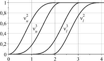
Figure 1. Upper ( u ) and lower ( / ) bounds of v³ (example for N = 3)

[t 3 , t p ] are obtained when integrating (9) forward from the point { v ³ } = { 0 } up to v ³ (t 3 ) = 1, then continuing with v ³ (t) = 1, and backward starting from the point {v ³ } = { 1 } . (this is illustrated in fig. 1 for the case N=3). Maximization of right hand sides is performed within these bounds v ^ (t), v ³ (t).

The following rather simple procedure is proposed to solve the optimization problem for the system (8) :

• 1.    Solve Cauchi problem for (8) backward starting from the point { v ^j } = { 1 } taking s ^j = — 1 up to v ^j (t j ) = 0 and recalculate the solution to the original time and variables y ^j .

• 2.    Solve (9) as was explained above to obtain the lower estimate of the transfer time t p .

For N = 2 and N = 3 the problem is solved directly and analytically.

N = 2: s1 = —1, v2 = 2/v 2(1 — v2), v2(0) = 0, v2 = (sin(t))2.

This coincides with solutions for N = 2 in [6] and also for Landau-Zener problem in [7] .

N = 3 : s ¹ = s ² — 1, v ⁴ = 0,

• (10)        v ² = 2 / (v ² — v ³ )(1 — v ² ), v ³ = 2 / (v ² — v ³ )v ³ ,

  /v ²     л/ (1 — v ² )

  /v ³       V v ³

  
  

  V v ³ + / (1 — v ² ) = C,

  
  

C = 1 for v ³ = v ² = 1 (and also for v ³ = v ² = 0). Then Vv ³ = 1 — ^(1 — v ² ). Substitution this into (10) leads to the single equation w.r.t. v ² (t)which has the following solution starting from v ² (0) = 0:

v ² (t) = 1 — (1/4)(1 + cos( V 2t)) ² ,   cos( V 2t _P )) = — 1, t _p = tt/V 2 .

This is minimal transfer time because the solution coincides with its lower estimate given by (9) . It is greater than that for N = 2 which is tt/ 2. The whole trajectory, recalculated to original variables is shown on fig. 2.

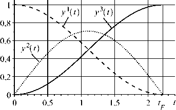
Figure 2. Exact solution for N = 3

For N >  3 there are no analytical solutions. However, it is possible to reduce and regularize calculation using the symmetry of (8) with given boundary conditions. Indeed, rewrite this system in new variables: £; ^k = 1 — л * , r ^k = — s * , к = N + 2 — j, j = 2,..., N when integrating from right to left:

C 2у^- ¹ i ^k )(i ^k    i ^{k +} )( ,r- 1 ), C =0, к = 2,...,N — 1,

This system is the same as (8) which means that it is sufficient to calculate (8) only from л * = 0 to л * =0.5 and to reconstruct the rest simply by symmetry. The overall time will be t(1) = 2t(0.5).

The following natural step in this investigation is to check whether this solution is realizable in the terms of system (5) . The values sin ((t i * ⁺¹ — y * ) — (h j+1 — h * )t ) = ± 1 imply cos ((y * ⁺¹ — y * ) — (h *+1 — h * )t ) = 0, and, further, from the equations w.r.t. y: 1 ¹ = 1, 1 * = 2, j = 2,..., that is

• 1 1    = 1 1 + t,  ¹1 ^N = т Г + t, Л³ = 1 * + 2t, j = 2, ...,N — 1.

• 4.    Conclusions

Then sin ((T2—1/)+t—(h2—h1)T) = —1, sin ((тГ1—1} ) — (hj+1—hj)t)) = —1.

It is possible to choose y * ⁺¹ — y * = — tt/ 2, j = 2,..., N — 1. Indeed, for example, taking t j = 0 implies y } = 0(given 6 j = 0); all the others y * ,j = 1 can be chosen arbitrarily due to singularity of the corresponding y * at y * = 0 (another question is how to implement this theoretical property). When defining h ₂ — h 1 = 1, h _r — h _r - 1 = 1, t = t, t >  0, (h *+1 = h * ), j = 2,..., N — 1, the equations w.r.t. y * are satisfied. Thus, all conditions of the first stage derived systems are satisfied. This means that the solution obtained is exact generalized one to the original system (3) and at least approximate one to the original problems on the minimum of the functional 1 — y(t p ) or minimum of trasfer time t p . The corresponding original control profile consists of two impulses at the endpoints (defined by t (0) and t (t _p ), and u(t) = 0 between the endpoints.

Application the special methods of degenerate problems theory allowed to obtain exact analytic solutions of the minimum time excitation transfer for the 2 - 3-spin chain model alternatively to laborious approximate computations with direct application of iterative methods to original problem.

For N -spin chains, N >  3, this results in rather simply computable solutions, which can be used as effective initial approximations in subsequent iterative improvement procedures. The ongoing research is oriented to construct such iterative procedures for sufficiently great amount of spins N with the use of various computational experiments and to clarification of the original real problem statement (real restrictions, control implementation, etc.) together with theoretical and practical physicists.