Two-dimensional mathematical models of visco-elastic deformation using a fractional differentiation apparatus

Author: Yaroslav Sokolovskyy, Maryana Levkovych
Journal: International Journal of Modern Education and Computer Science @ijmecs
Article in issue: 4 vol.10, 2018.
Free access
In this paper, using fractional differential and integral operators, constructed are two-dimensional mathematical models of viscoelastic deformation, which are characterized by memory effects, spatial non-locality, and self-organization. The fractal rheological models by Maxwell, Kelvin and Voigt, their structural properties and the influence of the fractional integro-differential operator on the process of viscoelasticity are investigated. Using the Laplace transform method and taking into account the properties of the fractional differential apparatus, analytical relations are obtained in the integral form for describing the stresses of generalized two-dimensional fractional-differential rheological models by Maxwell, Kelvin, and Voigt. Since the fractional-differential parameters of fractal models allow describing deformation-relaxation processes more perfectly than traditional methods, algorithmic aspects of identification of structural and fractal parameters of models are presented in the work. Explicit expressions have been obtained to describe the deformation process for one-dimensional fractional-differential models by Voigt, Kelvin, and Maxwell. The results of identification of structural and fractal parameters of the Maxwell and Voigt models are presented. The estimates of the accuracy of the obtained identification results were found using the statistical criterion based on the correlation coefficient. The influence of fractional-differential parameters on deformation-relaxation processes is investigated.
A mathematical model, derivatives of fractional order, rheological models, deformation processes
Short address: https://sciup.org/15016748
IDR: 15016748 | DOI: 10.5815/ijmecs.2018.04.01
Text of the scientific article Two-dimensional mathematical models of visco-elastic deformation using a fractional differentiation apparatus
Published Online April 2018 in MECS DOI: 10.5815/ijmecs.2018.04.01
The fractional integro-differential apparatus dates back to the birth of a differential calculus, so, today, in the theoretical aspect, it is well developed. However, despite this, the practical application of fractional derivatives and integrals for the description and study of physical processes has been started fairly recently and is becoming more and more relevant in various fields - technology [1], hydrology [2], physics [3], biology [4] , medicine [5] and others. Such interest can be justified by the fact that fractional differential operators allow us to describe the new properties of systems in comparison with systems that use derivatives of the integral order, which in turn allows us to describe and investigate more precisely models of the real world.
In the paper [6], a simple and optimal form of fractional-order feedback approach assigned for the control and synchronization of a class of fractional-order chaotic systems is proposed. In the paper [7] introduce the classical EOQ model with a linear trend of timedependent demand having no shortages using the concept of fractional calculus.
In the work [8] investigates the effectiveness of the physical-fractional and biological-genetic operators to develop an Optimal Form of Fractional-order PID Controller (O2Fo-PIDC). Implementation results are showed that the performance of the fractional-order PID controller is much better that PID controller and also instead of relatively complex and expensive controller, it is possible to use fractional-order PID controller for the problem [9].
The development of the idea of fractional integrodifferential apparatus for simulation of complex systems involves several scientific schools associated with the names: V. Uchaikin [10], A. Nakhushev [11], F. Mainardy [12], R. Nigmatulin [13], and I. Poddubny [14] and other scholars of the past and present.
Modeling the processes of viscoelastic deformation [10, 15-19] and heat-and-mass transfer [20-25] in environments with a fractal structure characterized by memory effects, spatial non-locality and self-organization must be also based on the use of the mathematical apparatus of fractional integro-differential operators. Fractional derivatives by time characterize the effects of memory (hereditament) or non-Markovian simulation processes, while fractional derivatives by spatial coordinates reflect the self-similar nonhomogeneity of the fractal environment.
Taking into account the mathematical apparatus of fractional integro-differential calculus and the structural properties of rheological models, one can obtain various fractal schemes of viscoelastic deformation which will describe bodies such as Jeffris’s, Maxwell’s, Kelvin’s, Voigt’s, etc.The use of differential equations of fractional order for constructing mathematical models of viscoelastic deformation allows for more adequate, based on physical considerations, the generalization of experimental data to identify model parameters [15].
One of the not completely solved problems is the problem of using the models of viscoelasticity of the fractional-differential type for constructing the corresponding phenomenological theories on the basis of known experimental data [26]. Classical identification methods have not been found to consistently provide the desired result when searching for fractal parameters. This can be explained by the fact that fractal parameters are often included in the Mittag-Leffler function, depicted as an infinite series. As a result of identification of finite numbers in the Mittag-Leffler series, we obtain a nonlinear system of algebraic equations, the solution of which is associated with large and laborious mathematical calculations. Taking into account the above, the identification of fractional-differential parameters requires some optimal non-classical method, or as is done in the work [26], the iterative method of coordinate descent is applied to the classical method of minimal squares.
To find the solution of integral and differential equations, both analytical [22, 23, 27] and numerical methods are used [17, 20, 21, 24, 25, 28, 29]. One of the applied analytical methods for solving fractional-differential equations is the Laplace transform method [10, 14, 27].
At present, a significant preference is given to numerical methods, since, as pointed out in [20], analytical methods for solving fractional diffusion equations are ineffective, and the theory of numerical methods for their solution is fragmentary and far from being complete. The numerical methods of current interest include the methods using finite-difference approximations [20, 21, 24, 25, 28, 29]. In the works [20, 21, 24] a numerical method is constructed using explicit and implicit difference schemes for solving onedimensional and two-dimensional heat-conduction problem with derivatives of a fractional order. An insignificant number of works [24, 25] is devoted to the study of boundary-value fractional order problems with boundary conditions of the third kind.
-
II. Problem Formulation
The basis of the simulation of two-dimensional deformation-relaxation processes in the fractal environment is the generalized classical theory of linear visco-elasticity and the properties of fractional- differential apparatus.
Maxwell’s fractal model (Fig. 1) is characterized by a series connection between the elastic element H and the viscous element N, while Voigt’s model (Fig. 3), on the contrary, is a parallel connection. Kelvin’s fractional differential model (Fig. 2) consists of a series connection of the Voigt body F and the elastic element H.
Taking into account the theory of the mechanics of hereditary environment [30-32], one can proceed from Kelvin’s fractal model to Maxwell's fractal model, taking away the elastic element, and thus taking that Ej = 0 . Thus, using various modifications of structural elements, various schemes of viscoelastic deformation can be obtained, which, in turn, can be described by differential equations of fractional order.
Non-fractal rheological models can be obtained by replacing the fractal element in the fractional-differential models with the viscous one. Given that viscocity n ( П = Етв , where E is modulus of elasticity, т is relaxation time, в is fraction order ( 0 < в < 1 ) ), and taking that в = 1 , we obtain classical rheological models.
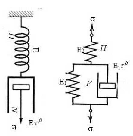
Fig.1. Maxwell's fractal model Fig.2. Kelvin’s fractal model
H
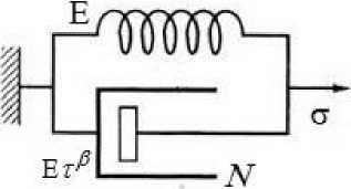
Fig.3. Voigt’s fractal model
Taking into account the above written, as well as the structural properties of rheological models investigated in [33] for the one-dimensional case, two-dimensional Voigt’s-, Kelvin’s-, and Maxwell’s models, with allowance for orthotropy in the fractal environment, can be described by the corresponding systems of equations:
Foigt’s model:
0-11 = С D.811 + С12 0.822 + 2Етв (Df8n + Df822),
^2 = C2Da8i + C22D822 + 2Etp (D^ + D8), a12 = 2C33Da^2 + Er^D;8^,
Kelvin’s model:
E a
T
O 11 + Dt O 11 = С 11 8 11 + С 12 8 22 +
( E 1 +E 2 )
+ HEE - ) ( ° ; 8" + D 8 ) •
(E 1 +e 2 )
- -
0 22 + 78 . x Dt 0 22 = С 21 8 11 + С22 ^ 22 +
(E 1 + E 2 )
в
+ tIS ( D ^n + D ' 6 22 ) ,
(E1 +E2 )
в
012 + DO = 2 С33812 +--1-2-
( E 1 +E 2 ) ( E 1 +E 2 )
Maxwell’s model
Oi + т“Д“О1 = С i8i + С 2812 + 2-2-в (Дв81 + Df 8,2) • cr22 + -4D o„ = С, 811 + С, 282 + 2-2 — (Dt 8\ + D 82) • ст12 + та Dao = 2 С3 382 + - 2 -}D! 8 2 ■ where 8T =( 8n, 822,812 ) • 7 = (on, 722, o12 ) is the vector of strains and stresses, components of which are dependent on time t and spatial variables x1 and x2, E, Ej, E2 are elastic modulus, Da, Dte are fractional derivatives in accordance with time and order, respectively a,в (for Voigt’s model - 0 < a < в < 1, for Kelvin’s and Maxwell’s - 0 < a, в < 1 ),
С , С , С , С , С are components of the elastic tensor for an orthotropic body, expressed through the formulas:
Ц - shear modulus, E1 p E22 - Young’ moduli, v , v " Poissons’s ratios
The fractional derivative in the sense of Riemann-Liouville order U of function f ( X ) can be written in the following way [10]:
x
f ( u ) ( x ) = F^j) D x i ( x - o- f ( ^ ) d ^ , ( )
0 < U < 1, Г ( - ) is Gamma function, Dx is an integer derivative of the first order variable x.
In the case where we put a = 0, in the relations (1) - (3), and a = в = 1, in (4)-(9), we obtain the classical twodimensional models by Voigt, Kelvin, and Maxwell in the orthotropic case, respectively.
-
III. A nalytical M ethod for R ealization of T wo D imensional M odels of V isco -E lasticity U sing F ractional D erivatives
The analytical relations in the integral form for describing strain-stress for rheological models are accomplished using the Laplace transform method and taking into account the fractional-differential apparatus and its properties. The following initial conditions are added to the above expressions (1) - (9):
° j - 1 )( 0 ) = a , 8 ( U - 1 )( 0 ) = bi , (12)
where ij = 11,22,12, a , bt are some constants.
Carry out the Laplace transform for Kelvin’s fractal model.
The solution of the corresponding system (4)-(6) reduces to finding a solution for each equation, for this we write as follows:
ла <7 j ( л ) + ( Е|+Е 2^ <7 j ( л ) = f ( л ) + C k , (13)
where k = 1,2,3 , fk ( 2 ) is Laplace’s pattern of the transformation of functions f ( t ) , which are as follows:
f ( 2 ) = (-1 1 V ; V;# (m 2 ) - 8 -( 2 ) ) + + V i-: ^ -™- ; .1 с- 6» ( л ) - 8 t 2 ( 2 ) ) +
p _ E 11 p _ v 2 E 11 p _ V 1 E 22
C” = ( 1 -vv 2 ) , C 12 = ( 1 v 2 ) , 21 = ( 1 -v , v 2 ) ,
+ 2 - 2 - e - a 2 e ( ( 8 11 ( 2 ) - 8 T 1 ( 2 ) ) + (. 8 22 ( 2 ) - 8 T 2 ( 2 ) ) ) ,
E 22 2 C 33 = ^ , (10)
22/1 \ , 33
( 1 - V 1 V 2 )
MX ) = ’га^(г„(. X ) - 6 „( X ) ) +
*(T- V^ ^ X ) " £ T ■ ( ^
+2E2re-“Xe ((6XX (X)- 6Ti (X)) + 6 (X)-6Т2 (X))), f3 (X)=(^ ( x)- ^ 3 ( x))+ <16>
+E 2E -“ Xе (s X 2 ( X ) - s т 3 ( X ) ) .
C are some coefficients that can be represented:
C X = С 2 = CTa - X )( o + ) - 2 E 2 Te - “ ( ^ в - 1 )( 0 + ) - 6 ^ - 1 )( 0 + ) ) +
+ ( ,( в - x ) ( 0 + ) -E ( в - x ) ( 0 + ) )
C 3 = CT ( a - x ) ( 0 + ) -Е 2 тв - “ 6 в - X )( o + ) - e ( в - X )( 0 + ) )
(17) where f a-X> (0 +) = lim ' [ f (§) d^.
-
1 ’ x ' 0 Г ( 1 - a )J ( x - §
Find transform of the solution:
Using the following relation in our case we obtain:
Y - X
L -1{ X- y } ( x ^
[10],
( ( E x +E 2 ) a
1 ^ I E,t“ a a , (Ex +E2)}(t ) = t ^, r(aj + a)
Ej T "
For further transformations, we use Mittag-Leffler’s two-dimensional function [34]:
to
E-(t >=E г(ой ■
The expression (21) can be rewritten in the following form:
L- {----- 7 --------?} ( t ) = t a -X E
E.+E2V()£
Xa + ( —
Ej T “
( E il E i) f ) (23>
E1 T “ J
Using the theorem on the resultant of two functions [10] and substituting the corresponding values of f k ( t ) and
Ck , we obtain the solution of the relations:
CT ij ( X ) =
f ( X )
X +
C^E^J. ^
E, T J
C k
X + ( Е 1 + Е 2 ) )
E, T1 J
t
CT 11 = С 1 G ( t ) + A J G ( t - O C n S 11 ( ^ )
0 -
+ 2 E 1 ! l Tв D ee 11(^ 1 d ^ +
( E 1 +E 2 )
t
To perform the inverse Laplace transform, it is convenient to apply the expression V| x" + (Ех +E2)) in / I Et J the form:
+ A J G ( t - ^ ) C 12 6 22 ( ^ ) +
t
| E1E¥ e D e£ 22 ( ^ ) ] d ^ ’ (e x +e 2 )
----1 г = X “ ---;------- X + (E 1 +E 2 ) X + (E 1 +E 2 ) x-“
Ej T Ej T
ct 22 = C 2 G ( t ) + A J G ( t - § ) C 21 6 ii ( ^ )
+ 2En Te D e6 11 ( § ) ] d § +
(E 1 +E 2 )
t
+ A J G ( t
- § ) C 22 6 22 ( § ) +
2 E i E 2 T i D ?6n ( ; )
( E 1 +E 2 ) t 22V ’
d § ,
to
=z j=0
(E.+E,)^ j
\ 1 2 X~“ j - “
E,^ J ’
Then:
t.
ct ,2 = C 3 G ( t ) + A J G ( t - § ) 2 C 33 6 ,2 ( § )
0 -
в
,E' E 2T , D ? 6. ( § ) d §
( E,+E2 ) t '2V ’
L {-------
X +
( E x +E 2 ) Ej T “
} ( t bZp E^ J L x j } ( t )
= 0 V E X T J
where
G ( t ) = t a - X E a a ( - At a )
A = ( E 1 +E 2 ) .
Ej T1
where L 1 is an operator of the inverse Laplace
transform.
Analytical formulas for the integral representation of Maxwell’s model can be obtained similarly by solving each equation from the system (7)-(9) by the Laplace transform method, or from Kelvin’s model, putting in the relations (24>-(26> that E, = 0 ■
The relationship between stresses and deformations for Maxwell’s fractional-differential model in an integral form can be represented as follows:
° 11 = C 1 F ( t ) + 4 f F ( t - 5 ) [ c 1 £ 11 5 ) + 2 E 2 re D f £U ( 5 ) d +
T 0
+ 4 J f ( t - 5 ) [ C 12 ^ 22 ( 5 ) + 2 E 2 Te D eE 22 ( 5 ))/ 5 ,
T 0
° 22 = C 2 F ( t ) + 4 J f ( 1 - 5 ) [ c 2 £ 11 ( 5 ) + 2 E т Ч > в£. 1 5 ^5 + T 0
+ 1 - J f ( t - £ ) C 22 £ 22 ( ^ ) + 2 Е т Ч.-; 22 ( 5^5 ,
T 0
° 12 = C 3 F ( t ) + ^ J f ( t -5 ) [2 C 33 ^ 2 ( 5VV ; : D £ 2 ( 5 )] d ^
T 0
where i a ^
F ( t ) = t a E aa [- "a J .
IV. Identification of Fractal Parameters of Models and Analysis of Numerical ModelingResults
For one-dimensional fractional-differential models of Voigt, Kelvin, and Maxwell, the explicit form of the expression describing the deformation can be represented as follows:
£ ( t ) = — «° 0 / x [2 1 в -( t - tY )в hit - t )!-
F () Е т в в Г ( в )L ( 1 ) ( 1 )J
- Е т2 в-a ( 2 в - 0 ) Г ( 2 в -« ) [ 2 t2 ва -( t - t 1 ) в h ( t - t 1 ) ] ,
£K (1) =
(Е 1 +Е 2 ) ° 0 Е , Е 2 т в в Г ( в )
( Е 1 +Е 2 ) ° 0 Е,Е2 т 2 в 2 в Г ( 2 в )
J2 1 в -( t - t 1 ) в h ( t - t 1 ) ]
J2 t 2 в -( t - t 1 ) 0 h ( t - t 1 ) ]
+__________ ° 0__________ Г 1 в-"
Е2 т в-а Г ( 1 - а ) Г ( в ) 1
+
-(1 -11) в h (1 -11)]-
____________° 0____________ Г/ 2 в - а
Е2 т2 в Г ( 1 а ) Г ( 2 в ) 1
-( 1 - t 1 ) в h ( 1 - t 1 ) ],
£ M ( 1 ) = Е т 0 0 Г ( в ) [ 2 1 в " ( 1 - 1 1 ) в h ( 1 - 1 1 ) ] +
For the integral representation of the relations (1)-(3), the properties of fractional derivatives [10, 34, 35], as well as the relation (11) are taken into account. As a result of the appropriate transformations, we obtain the analytical relations for stresses in the integral form for Foigt’s fractal model:
+ ° v^? Г2 1 в-а Е т в - а ( в - а ) Г ( в - a ) L
- ( t - t 1 ) в-а h ( t - t 1 ) ],
° 11 =
E 11
( 1 - v 1 v 2 ) r ( 1 - a )
t
D t J ( t к 0
^
- 5 ) “ [ £ 11 ( 5 ) + v 2 £ 22 ( 5 ) ] d 5
J
+
+
В i
^(^ ^ D t J ( t - 5 )- в £ 11 ( 5 ) + £ 22 ( 5 ) ] d 5
° 22
E 22
( 1 - v 1 v 2 )r( 1 - « )
i D t J ( t
к 0
- 5 ) a [ v 1 £ 11 ( 5 ) + £ 22 ( 5 )] d 5 + J
2 Ет в
+ Г ( 1 - в )
i )
D t J ( t - 5 ) в [ £ 11 ( 5 ) + £ 22 ( 5 ) ] d5 .
к 0 J
where ° is the value of the stress at the initial time , h ( t ) is Heaviside function ( h ( t ) = 0 at t < 0, h ( t ) = 1at t > 0 ), t is unload time.
The task of identification is divided into two subtasks: identification of structural parameters (elastic modulus, relaxation time, viscosity, initial stress, etc.), identification of fractional-differential parameters of models a and в .
Since the structural parameters of fractional-differential rheological models a priori should coincide with the structural parameters of the classical rheological models, we will identify these parameters using the creep law for a specific model in its classical interpretation.
Tus, let us present the law of creep for models:
Voigt’s model:
° 12
=Dt J
^ ( 1 - 5 ) - “ Г( 1 - «a
Е тв ( t - 5 ) - в ) г ( 1 - в ) Jf12
( 5 ) d 5 (32)
£ (1 ) = ° (1 - e-X), (36)
Kelvin’s model
4 ( t ) =
Ej+E2 E 1 E 2

P " =
To express the creep equation for Maxwell’s model, as was done in the previous cases for Kelvin’s and Voigt’s models, is not possible in the classical theory. This is explained by the fact that, putting r = const in the Maxwell equation, we obtain d " (t ) = -^ . It follows t v 7 Et that the Maxwell body under the action of constant stress will flow as a Newtonian fluid with a constant rate of deformation [31].
Taking into account the above written, in order to find the structural parameters of Maxwell’s model, we use the deformation equation that describes Maxwell’s fractional-differential model while assuming that the fractional parameters a , в are equal to one.
E ( "i- "avg )( " - "avg ) i = 0
where " , " are deformation values for each model
according to the obtained expressions and experimental
data , " avg
1
n + 1
n
E "i, "avg i=0
1
n + 1
n
E s.
i = 0
Here are the results of the identification of structural
( r , T ) and fractal ( a , в ) parameters for Maxwell’s model (Fig. 4) and Voigt’s one (Fig. 5) at ambient temperature T = 23 ° C .Using the experimental data [36], Maxwell’s model was investigated for specimen No. 6, and Voigt’s model – for No. 57 (Table 1).
"M ( t ) = r [ 4 1 - 2 ( t - ' 1 ) h ( t - 1 | ) ] • (38)
Having a sample of experimental values [36] "k к м ( t ) = " using the method of minimum squares, we minimize the deformation functions of the models:
n
E"-"F,к,m (t,TrE)) ^min. (39) i=1
Assuming that the structural parameters in the relations (33)-(35) were found, the values of fractional-differential parameters are identified by minimizing the deformation functions. To do this, using the method of minimum squares and having a set of experimental data [36], we can write :
E" - "f, K, M ( ti,a, в)) ^ min.
i =1
In order to clarify the identification parameters, the method of coordinate descent [26] was used.
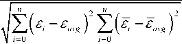
For the quantitative estimation of the difference between the results obtained for the fractional-differential creep equations (33)-(35), a statistical criterion based on the correlation coefficient was used.
The criterion looks like:
A = ,1 P " V n - 2, (41)
Ji- P "
where n is the number of points for which the comparison of values is made, P " is the correlation coefficient, which is determined by the ratio:
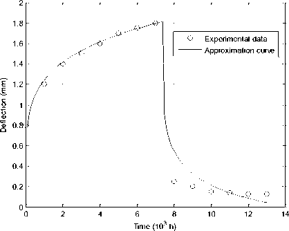
Fig.4. Identification of fractional-differential parameters of Maxwell's model
Table 1.Values for identification parameters, criterion and correlation coefficients.
|
Identification parameters, criterion value |
Specimen No. 6, E = 15.3(10 3 M pa ) W= 30 % |
Specimen No. 57, E = 17.3(10 3 M pa ) W= 7.5 % |
|
r 0 (103 M pa ) |
3.1424 |
4.2859 |
|
T (10 3 h ) |
0.1804 |
6.8769 |
|
a |
0.0024 |
0.1858 |
|
в |
0.1922 |
0.1867 |
|
P |
0.9921 |
0.6891 |
|
A |
26.15 |
3.153 |
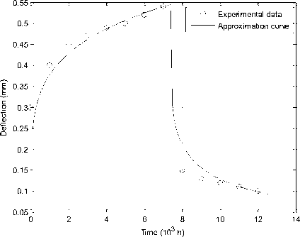
Fig.5. Identification of fractional-differential parameters of Voigt’s model
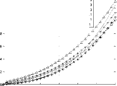
1.4
beta=0.7,alpha=0.1
alpha=0.7, beta=0.9 alpha=0.5, beta=0.9 alpha=0.3, beta=0.9 beta=0.3, alpha=0.1
1.2
E E
1 1.5 2 2.5
Time (h)
Fig.6. Dependence of Voigt’s model on fractal parameters
A numerical experiment to determine the dependence of deformation £ ( t ) (Fig. 6) and stress a ( t ) (Fig. 7) for fractal models was carried out as follows. For the following species of wood such as oak and pine, the moduli of elasticity of which are respectively (Eoat = 14300 M pa , Epine = 12100 M pa ) ,it is determined how the deformation and stress at different and fixed fractional differential parameters of the models will change. For example, for Voigt’s model, the fractal parameter a is fixed closer to 0 ( а = 0.1 ), with в being variable, and vice versa в is fixed closer to 1 ( в = 0.9 ), with a being variable. On analyzing the results obtained, it can be noted that at the fixed parameter а = 0.1 with an increase in the fractional-differential parameter в , the value for the deformation decreases, however, at the fixed fractal parameter в = 0.9 , the value for the deformation increases as the parameter a increases.
Fig. 7 shows stress curves for Maxwell-Kelvin-type fractional-differential models for a fixed parameter в = 0.9 and a variable parameter а where а = 0.2 + Aa , Aa = 0.3 . It is obvious from graphic dependences that for both models the smallest value for stress is reached at a = 0.8, and the largest - at a = 0.2.
Since the Maxwell model can be obtained from the Kelvin model, as shown above, and vice versa, the Kelvin model, by modifying and adding another elastic element, can be obtained from the Maxwell model, from the graphic dependences it can be concluded that the curves are quite close to each other. Thus, at some point in time, the stress values for the Kelvin and Maxwell fractal models coincide.
The Maxwell model (alpha=0.2)
The Maxwell model (alpha=0.5)
The Maxwell model (alpha=0.8)
The Kelvin model (alpha=0.2)
The Kelvin model (alpha=0.5)
The Kelvin model (alpha=0.8)
0 0.5
1 1.5 2 2.5
Time (h)
Fig.7. Dependence of Maxwell’s and Kelvin’s models on fractal parameters
-
V. Conclusions
Taking into account the fractional-differential apparatus, two-dimensional mathematical models of deformation-relaxation processes in fractal environments have been constructed. For the fractional-differential models of Maxwell, Kelvin, and Voigt, expressions describing the stresses in the integral form are found. The identification of fractal parameters and the criterion of error estimation are given. Investigated and analyzed is the influence of fractal parameters on the rheological properties of viscoelastic environments.
References Two-dimensional mathematical models of visco-elastic deformation using a fractional differentiation apparatus
- Machado, J.A.T., Galhano, A.M.S.F., “Fractional order inductive phenomena based on the skin effect” Non-linearly. Dyn. 68(1–2), pp. 107–115, 2012.
- Sheng, H., Chen, Y.Q., Qiu, T.S., “Fractional Processes and Fractional-Order Signal Processing”, Springer, New York, 2012.
- Mohamed A. E. Herzallah, Ahmed M. A. El-Sayed, Dumitru Baleanu, “On the fractional-order diffusion-wave process”, Rom. Journ. Phys., vol. 55, Nos. 3-4, pp. 274-284, 2010.
- F. A. Rihan, D. H. Abdel Rahman, S. Lakshmanan, and A. Alkhajeh, “A time delay model of tumour—immune system interactions: global dynamics, parameter estimation, sensitivity analysis,” Applied Mathematics and Computation, vol. 232, pp. 606–623, 2014.
- Y. Ferdri, “ Some applications of fractional order calculus to design digital filters for biomedical signal processing’, J. Mech. Med. Biol. 12(2), p. 13, 2012.
- Ammar Soukkou, Salah Leulmi,"Controlling and Synchronizing of Fractional-Order Chaotic Systems via Simple and Optimal Fractional-Order Feedback Controller", International Journal of Intelligent Systems and Applications(IJISA), Vol.8, No.6, pp.56-69, 2016. DOI: 10.5815/ijisa.2016.06.07
- Asim Kumar Das, Tapan Kumar Roy,"Fractional Order EOQ Model with Linear Trend of Time-Dependent Demand", IJISA, vol.7, no.3, pp.44-53, 2015. DOI: 10.5815/ijisa.2015.03.06
- Ammar Soukkou, M. C. Belhour, Salah Leulmi, "Review, Design, Optimization and Stability Analysis of Fractional-Order PID Controller", International Journal of Intelligent Systems and Applications(IJISA), Vol.8, No.7, pp.73-96, 2016. DOI: 10.5815/ijisa.2016.07.08
- O. Tolga Altinoz, A. Egemen Yilmaz, "Optimal PID Design for Control of Active Car Suspension System", International Journal of Information Technology and Computer Science(IJITCS), Vol.10, No.1, pp.16-23, 2018. DOI: 10.5815/ijitcs.2018.01.02
- V. Uchajkin, “Method of fractional derivatives”, Ulyanovsk: Publishing house «Artishok», p. 512, 2008.
- A. M. Nahushev, “Fractional calculus and its application”, Moscow: Fizmatlit, p. 272, 2003.
- J. Tenreiro Machado, V. Kiryakova, F. Mainardi, “Recent history of fractional calculus”, Commun Nonlinear Science and Numer Simulat., vol. 16., pp. 1140-1153, 2011.
- R. R. Nigmatullin, “Fractional integral and its physical interpretation”, Theoretical and Mathematical Physics, T. 90, No. 3., 1992, pp. 354-368.
- I. Podlubny, “ Fractional Differential Equations”, of Mathematics in Science and Engineering, Academic Press, San Diego, Calif, USA, vol. 198, p.340, 1999.
- S. V. Erokhin, T. S. Aleoev, L. Yu. Frishter, A. V. Kolesnichenko, “Parametric identification of the mathematical model of viscoelastic materials using fractional derivatives”, International Journal of Computational Civil and Structural Engineering, vol. 11, Issue 3, pp. 82-85, 2015.
- S. V. Erokhin, “Models of creep and relaxation of materials using fractional derivatives”, Construction mechanics of engineering structures and structures, No. 6 Moscow, pp. 35-39, 2014.
- M. Javidi, B. Ahmad, “Advances in Difference Equations”, p. 375, 2013.
- N. W. Tschoegl, “The Phenomenological Theory of Linear Viscoelastic Behavior”, Berlin, Springer, 1989.
- E. N. Ogorodnikov, V. P. Radchenko, N. S. Yashagin, “Rheological models of a viscoelastic body with memory and differential equations of fractional oscillators”, Vestn. Himself. state tech un-that Sir Fiz. Mat. science, No. 1 (22), pp. 255-268, 2011.
- V. D. Beibalayev, “Mathematical model of heat transfer in mediums with fractal structure”, Mathematical modeling, vol. 21, No. 5, pp.55-62, 2009.
- V. D. Beybalaev, M. R. Shabanova, “Numerical method for solving the boundary value problem for a two-dimensional heat equation with derivatives of fractional order”, Vestn. Himself. state tech un-that Sir Fiz. Mat. Science, №5 (21), pp. 244-251, 2010.
- R. P. Meilanov, M. R. Shabanova, “The equation of thermal conductivity for media with fractal structure”, Modern science-intensive technologies, No. 8, pp. 84-85, 2007.
- R. P.Meilanov, M. R. Shabanova, “Features the solution of the heat transfer transport equation in derivatives of fractional order”, Journal of Technical Physics, Vol. 8, Issue 7, pp. 1-6, 2011.
- A. K. Basayev, “Local-one-dimensional scheme for the equation of thermal conductivity with boundary conditions of the third kind”, Vladikavkaz Mathematical Journal, Vol. 13, Issue 1, pp. 3-12, 2011.
- Ya. Sokolowskyy and V. Shymanskyi, “Mathematical modeling of non-isothermal moisture transfer and rheological behavior in capillary-porous materials with fractal structure during drying”, Computer and Information Science, Canadian Center for Science and Education, Vol. 7, No. 4, pp. 111-122, 2014.
- Е. Ogorodnikov, V. Radchenko, L. Ugarova, “Mathematical modeling of hereditary deformational elastic body on the basis of structural models and of vehicle fractional integral-differentiation Riman-Liuvil”, Vest. Sam. Gos. Techn. Un-ty. Series. Phys.-math. sciences, tom 20, number 1, pp. 167-194, 2016.
- L. Kexue, P. Jigen, “Laplace transform and fractional differential equations”, Appl. Math. Lett., 24, pp. 2019-2023, 2011.
- N. J. Ford, A. C. Simpson, “The numerical solution of fractional differential equations: speed versus accuracy”, Numer. Algorithms, 26(4), pp. 333-346, 2001.
- K. Diethelm, “An algorithm for the numerical solution of differential equations of fractional order”, Electron. Trans. Numer. Anal. 5, pp. 1-6, 1997.
- G. M. Savin G., “Elements of the mechanics of hereditary environments”, Rheological bodies with the simplest law of linear deformation , No. 1, p.114, 1969.
- G. M. Savin, “Elements of the mechanics of hereditary environments”, Rheological bodies with the simplest law of linear deformation, No. 2, p.137, 1970.
- G. M. Savin, Ya. Ya. Ruschytsky, “Elements of the mechanics of hereditary environments”, The textbook for the mechanics and mathematics faculties of universities, K. -"High School", p. 251, 1976.
- Ya. I. Sokolovsky, M. V. Moskvitina, “Mathematical modeling of deformation-relaxation processes using derivatives of fractional order”, Bulletin of the National University "Lviv Polytechnic", Computer Science and Information Technologies. No. 826. - Lviv: NU "LP", pp. 175-184, 2015.
- V. V. Vasilyev, L. A. Simak, “Fractional calculus and approximation methods in the modeling of dynamic systems”, Scientific publication Kiev, National Academy of Sciences of Ukraine, p.256, 2008.
- S. G. Samko, A. A. Kilbas, O. I. Marichev, “Integrals and derivatives of fractional order and some of their’, Minsk: Science and Technology, p. 688, 1987.
- Tong Liu, “Creep of wood under a large span of loads in constant and varying environments", Pt.1, Experimental observations and analysis, Holz als Roh- und Werkstoff 51, pp. 400-405, 1993.
