Two-Dimensional Parameters Estimation

Published Online September 2016 in MECS

The applications of high-resolution parameters estimation span a wide domain ranging from detection to surveillance. The two methods used to accomplish this are spectral based approach and parametric approach [1]. Speaking in the context of MUSIC, it is a high-resolution subspace based technique falling under the category of spectral based approach which utilizes covariance matrix to estimate the parameters of interest. MUSIC [2], [3] has a very high resolution and it assumes noise to be uncorrelated which leads to the diagonal correlation matrix. As a major drawback [4] MUSIC cannot be termed as a general approach as it requires advance information about the number of elements.

Estimation of Signal Parameter via Rotational Invariance Matrix (ESPRIT) [5] is also based on subspace-based approach and is a key contributor to the estimation theory. ESPRIT again is a high-resolution parameter estimation technique and has the additional advantage of lesser computational complexity. Its assumptions include sources to be centered at the same particular frequency and doublets of arrays that are not displaced rotationally [6], [7].

Parametric approach methods include Least Square Estimation (LSE) and Maximum Likelihood Estimation (MLE) [8], [9]. The maximum-likelihood method unlike least square method which models the estimation problem as a deterministic procedure demands probabilistic interpretation of all the interferences rather than the information of the parameters. Also, MLE output the parameter that is most likely responsible for producing data while LSE shortlists the parameter that seems to be the closest interpretation of the received data.

But, MLE estimates differ from LSE estimates when received data is not normally distributed and uncorrelated and different results are obtained depending upon the choice of the method between the two. However, in such a scenario MLE is preferred over LSE if probability distribution function description of the data is available. Also, both MLE and LSE arrive at same estimates if the data is normally distributed with constant variance [10], [11], [12].

In this paper, a MLE based algorithm is proposed for the estimation of different parameters of moving targets using electromagnetic sensor array. MLE suffers the disadvantage of higher computational complexity because it spans the entire signal space but has the side advantage of high-resolution parameter estimation even when the received data is corrupted by correlated noise, a condition under which MUSIC fails.

The rest of the paper is organized as follows. Section II deals with the problem formulation and derivation of the data model for the proposed algorithm. In section III, the developed data model is used for parameters estimation (DOA and velocity) using MLE. Section IV covers the simulations used for the verification of the algorithm. In section V, the MUSIC is discussed briefly and simulations are carried out to analyze the performance of the MUSIC under different circumstances with a motive of comparison between MUSIC and developed algorithm. Section VI discusses the Cramer- Rao bound, its role in the classification of the different estimators and Cramer-Rao bound calculation for the present algorithm. Section VII finally concludes the observations and results of the paper.

• II.    Data Model

For the illustration of the proposed algorithm, the discussion to be considered here is focused on DOA and velocity estimation. In signal processing, for solving such a problem, the sensors array is deployed to collect the data from the radiating sources for estimating their different parameters. Few assumptions are further invoked for the analytical compliance of the problem. The radiations from the sources are assumed to be propagating in straight lines. A dispersive and isotropic transmission medium is required to validate the above assumption. Also, the radiations striking the array can be considered as plane waves if sources are within the far-field of the array. The narrowband signals ( s ( t )) are assumed to have center frequency ( to ) so that the general wave equation is given as:

E ( r , t ) = 5 ( t ) Re[e (^ ^{- k . r )} ]            (1)

where k is propagation vector and r is position vector.

¥

x ( r , t ) = y ( 9 ) 5 ( t ) Re [ e ^{( m} " t ^— k ^{( l — 1) d cos 9} ]       (2)

Also, to₀ will get shifted according to Doppler’s classical shift formulae i.e. to = to (1 — v / c )

Then, the output of l^th sensor after dropping the term e*™⁰¹ gets modified to:

x ( r i , t ) = y ( 9 ) 5 ( t ) e ^{— j to vt} / ^c

— jk ( l — 1) d cos 9

In case of L sensors ULA, having same response for all sensors i.e. y ( 9 ) = y ( 9 ), the output can be represented as a vector

x ( t ) = 5 ( t ) e ^{— j to vt} / ^c a ( 9 )               (4)

where,        x( t) = [ x (t) x2 (t) . . xL (t)]        and ag = y(9)[1 e—jkdcos9 . . e—j(L—1)kdcos9] which is also called steering vector. Consider the case of p sources each located at an angle 9 . If the medium is considered to be linear then the output of each sensor can be written as:

x_L ( t ) = 5 ( t ) y ( 9 ) e ^—' / ^c e ^{— jk ( L — 1) d cos 9 1}

+ s ₂ ( t ) y ( 9 ) e ^— ^' / ^c e ^{— jk ( L — 1) d cos 9 2}

+ s_p ( t ) y (9, ) e ^{— jv to} ‘ / ^c e ^{— jk} ( L ^— 1) d cos ^{9 p}

If the sensor’s response is same for every source i.e. y ( 9 ) = y( 9 ) = y(9_p ) = y ( 9 ) then the above equation can be written as:

x ₁ ( t )

x ₂ ( t )

— jkdcos 9 e ¹

— jkdcos 9

e ²

— jkdcos9_p

= y ( 9 )

X

- ^X l ( ‘ ) -

— jk ( L — 1) cos ^

— jk ( L — 1) cos ^

— jk ( L — 1) cos9p

• • - • « •-----------------* —► X

o d Id 3d                   (L-Y)d

Fig.1. Uniform linear array

If we have a uniform linear array (ULA) [13] having L sensors and separation d between them (Fig. 1), then position vector at the Vh sensor is given as r = (l — 1)da. Consider the case of a source moving with velocity v and having a component along the direction of the line joining the origin and impinging angle 9 at the Vh sensor having a       constant       response      y (9).      Then, k = cos 9a + sin 9a and output of the sensor is given as: xy s, (‘) e—jtoV1‘ / c s2 (‘) e ""'2 ‘"

s_p ( t ) e

— j to Vpt / c

It can be represented as:

x ( t ) = A ( 9 ) s v ( t )                  ⁽⁵⁾

Taking sensor’s noise into consideration:

x ( t ) = A ( 9 ) s _v ( t ) + n ( t )             (6)

If the sensor’s output is sampled at t = m S where m = 0,1....... k — 1 then:

x ( m S ) = A ( 6 ) s_v ( m S ) + n ( m S )     (7)

From above equation the output for the l^th sensor can be written as:

x, ( m S ) = ^Л ( m S ) e - ^{j ( 1 — 1)} d cos ⁶ .e^{JjOm S} / c   (8)

n = 1

If 8_И ( m S ) = S_n , the above equation can be rewritten as:

p

X 1 = Z S n e ( 6 n ) 0 f ( V n ) + W |         (9)

n = 1

here X represents the time samples of the sensor output x .

Also e6) = [ e

— jk ( 1 — 1)cos 6 ,,

]

and e - jSvn / c e -j 25vn / c f (Vn ) = e - j (k -1) Svn / c

This concept can be extended to all the sensors and the resulting output can be written as:

p

X = E ^sn e ^{( 6} n ) ^{0 f (} V n ) ⁺ w        ⁽¹⁰⁾

n = 1

here

e ( 6 n ) = [1

— jkd cos 6

e — j ( L — 1) kd cos 6 n ] T

The above equation can also be written as:

X = S[e(6) 0 f (V1)  e(62) 0 f (v2)  .  .  e(6p) 0 f (vp)] + W where

S = [ S S 2   .  . S p f

We define

A ( n ) = [ e ( 6 ) 0 f ( v , )    e ( 6 ₂) 0 f ( v ₂)   .   .    e ( 6_p ) 0 f ( v_p )]

here S is p x 1 and A ( n ) is Lk x p matrix. Using above representations, the final form of the data model is:

X = A ( n ) S + W             (11)

• III.    Parameter Estimation

In the data model signal waveforms are assumed to be deterministic but unknown and noise is modelled as i.i.d. spatio-temporal white Gaussian random process with constant variance i.e.        ²     . As a result X is also a

Lk x 1

Gaussian random process with mean A ( n ) S and variance о ² I . The PDF of a Gaussian random variable is given by:

p ( x ) = —--- e -^{( x} - ^ ^)2/2 ° 2          (12)

V 2 по о

Here ц and о ² represent mean and variance of the random variable. Using (12), the PDF of observation vector X is given by:

Y = ce—lix—A(n)S||2/2o2^^

where, C is a constant and does not contribute to decision making. Taking log of both sides of (13), we get

Z = —     ||X — A(n)S ||2

Neglecting the term _— C , we get PDF as: 2 o²

Y =|| X — A(n)S ||2

The maximum-likelihood estimation rule dictates that (15) is to be minimized with respect to n . First, to obtain maximum-likelihood (ML) estimate of S , the derivative of (15) with respect to S is set to zero. This will result in

5 ' = ( A^HA ) ^{— 1} A ^H X            (16)

where A is a function of n . Using (15) and (16), we get

Y = || X — P ( n ) X||²                  (17)

where P( n ) = A(A H A ) ¹ A H . The above expression can be rewritten as:

Y=( IMI2 -IP(n)MГ )             (18)

Minimizing the above expression implies maximizing! | P ( n ) M ||². So, the ML estimate of parameter П is given by:

П = Arg max _n |P ( n ) M||^{2 (19)}

The MLE estimate can be determined by exploiting the non-linear optimization algorithms. The basic principle behind non-linear optimization is to find the optimal parameters so that log-likelihood function is maximized [14]. This can be achieved by dividing the multi-dimensional parameter space into smaller sub-sets and applying trial and error approach such that for next iteration parameters value is modified so that it leads to better performance than that for previous parameters values.

0.5     0.6     0.7     0.8     0.9       1       1.1      1.2     1.3      1.4

Direction in radians

Fig.2. Direction estimation of the first target at 10dB

2.5

Noise effect

Ideal

IV. Simulations

Many simulations have been conducted to explore the various aspects of above discussed algorithm. The numbers of sensors on the array were chosen to be five with uniform spacing between them. Also, the centre frequency was chosen as 100* c , where c _the velocity of light. The sampling interval 5 was chosen to be equal to the wavelength ( Я ) of the signal. The spacing ( d ) between

0.4    0.6    0.8     1     1.2    1.4    1.6    1.8     2     2.2    2.4

Direction in radians

sensors was chosen to be X /10 . Also, the numbers of targets were chosen to be two and it was also assumed that numbers of targets are known in advance. The noise was assumed to be additive white Gaussian noise with zero

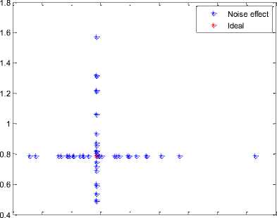
Fig.3. Direction estimation of the second target at 10dB

B. Velocity Estimations of the Targets

mean and unit variance. Also, the velocity of targets was

restricted between 1/50 to 1/10 m/sec i.e.

v =

50,10

Targets were having a velocity of 1/40 and 1/20 m/s. Other conditions were same as for direction estimation. Estimations are illustrated in Fig.4 and Fig.5.

m/sec., however, no restriction was made in the direction of targets i.e. 0 = [0, 2 n ] radians.

0.032

0.03

Noise effect Ideal

• A. Direction Estimations of Targets

0.028 0.026 0.024 0.022 0.02 0.018 0.016 0.014 0.01 0.015         0.02         0.025         0.03         0.035

Two targets were located at π/4 and π/2 radians respectively and were of unequal power. Also, the signal to noise ratio (SNR) for each target was 10dB and 51 iterations were conducted, one for estimation under the ideal condition and other 50 for estimation when the noise was present. In each trial noise was different. Estimations are illustrated in Fig.2 and Fig.3.

Velocity in m/sec

Fig.4. Velocity estimation of the first target

E

0.08

0.07

0.06

0.05■к

0.04

0.03

0.02

0.01

*-

t

*-   Noise effect t-   Ideal

0.0265

0.026

0.0255 E

0.025

0.0245

*- Noise effect

*• Ideal

*                       *■

0     0.01   0.02   0.03   0.04   0.05   0.06   0.07   0.08   0.09

Velocity in m/sec

Fig.5. Velocity estimation of the second target

0.024t---------------Г---------------^---------------Г----------------1---------------1

0.024        0.0245       0.025        0.0255       0.026       0.0265

Velocity in m/sec

Fig.8. Velocity estimation of the first target at 20 dB

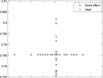
Another 51 iterations were made for these two targets with SNR of 20 dB. Results are shown in Fig.6, Fig.7, Fig.8 and Fig.9.

0.055

0.765    0.77    0.775    0.78    0.785    0.79   0.795    0.8    0.805

Direction in radians

Fig.6. Direction estimation of the first target at 20 dB

0.054

0.053

0.052

0.051

0.05

0.049 к                                *.

1.58

1.555

1.56

1.575

1.57

1.565

1.56

	---------------1----------------------------
	4="   Noise effect
	*   Ideal
	*" * *"

1.565

1.57

1.575

1.58

Direction in radians

1.585

Fig.7. Direction estimation of the second target at 20 dB

*• Noise effect

*- Ideal

0.048 t---------------r---------------1--------------^--------------1--------------r---------------1

0.047      0.048      0.049       0.05      0.051      0.052      0.053

Velocity in m/sec

Fig.9. Velocity estimation of the second target at 20 dB

Simulations depict the validity of the algorithm for ideal case and to a greater extent for practical scenario as well (presence of noise). Also, it can be observed that effect of noise is less prominent in case of velocity estimation as compared with the case of direction estimation. Further, the average error in estimations for different SNR is summarized in table 1.

Table 1. Average error in parameters estimation

SNR	Error in direction estimation	Error in velocity estimation
10dB	.65	.034
20dB	.011	.033

C. Effect of enhanced SNR on estimation error

Fig.10 and Fig.11 depict the effect of SNR on error in estimations.

Error in direction estimation of first target

Fig.10. Effect on direction estimation

_{x 10}^-3                                                                          Error in velocity estimation

• 4.5

• 3.5

• 2.5

0.5

10              11              12              13              14              15              16              17              18              19              20

SNR

Fig.11. Effect on velocity estimation

It is observed from Fig.10 and Fig.11 that performance of the algorithm is improving drastically with improvement in SNR and theoretically at very high SNR the algorithm will achieve noise immunity.

• V. MUSIC Estimator

For the sake of completeness and for demonstrating the pragmatic aspect of the developed algorithm, a comparison with MUSIC estimator is made in this section. MUSIC was introduced as a most effective DOA estimation technique which proceeds by decomposition of covariance matrix and forming a spectrum using steering vector. MUSIC works well for ideal case and uncorrelated noise but fails for the correlated noise.

Reconsider the data model

x ( t ) = A ( θ ) s _v ( t ) + n ( t )

We define spatial-covariance matrix as:

R = E { x ( t ) x ^H ( t )}

R = A ( θ ) E { s v ( t ) s v^H ( t )} A ^H + E { n ( t ) n ^H ( t )}

If noise is assumed to be spatio-temporal white with common variance σ ² then

E{n(t)nH(t)}=σ2I and if P = E{s (t)s H (t)} then R will become

R = A ( θ ) PA ^H ( θ ) + σ ² I

R can be factored as R = U Λ U^H  with

Λ = diag[λ λ .  . λ ] is a diagonal matrix of eigen values λ,λ ,...λ and U is a unitary matrix having eigen vectors corresponding to eigen values λ,λ,...λ . R can also be written as

R=UsΛnUsH +UnΛnUnH(20)

with Λ = σ ² I . In practise, an estimate of R is found as

R=1∑k x(t)xH(t)

k t = 1

Hence,

Rs =UsΛsUsH+UnΛnUnH(22)

The projector operators onto signal subspace are defined as:

Π=UsUsH=A(θ)(A(θ)HA(θ))-1A(θ)H(23)

Similarly, projection onto noise signal subspace is defined as:

Π ^⊥ = U_nU_n^H = I - A ( θ )( A ( θ ) ^H A ( θ )) ^{- 1} A ( θ ) ^H (24)

The MUSIC spatial spectrum is then defined as:

_{P ( θ ) =} a ^H ( θ ) a ( θ )

^M     a ^H ( θ ) ∏ ^⊥ a ( θ )

Where, a ( θ ) is steering vector.

P ( θ ) is not a true spectrum but instead gives a peak at the point of direction of arrival (DOA).

• A. Simulations

Several simulations were carried out to analyse the performance of MUSIC algorithm and to compare it with the developed algorithm for the case of (DOA) estimation. Two sources were chosen in the far field of sensors array which were located at π/3 and π/2 radians. Also, the numbers of sensors were chosen to be five. Few simulations were carried under ideal conditions (absence of noise) and then under uncorrelated noise conditions. Simulations were also carried for correlated noise with different SNR.

X: 1.047

Y: 1

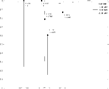
1.5                2

Direction of Arrival

Fig.14. Estimation under correlated noise for different SNR

Direction of Arrival( in radians)

Fig.12. Ideal estimation

Direction of Arrival (in radians)

Fig.13. Estimation under uncorrelated noise

It can be inference from the simulations that MUSIC and proposed algorithm are contrasting for the case of correlated noise. The performance of MUSIC is compromised drastically for this case but for ideal case and uncorrelated noise MUSIC is always way ahead of the proposed algorithm considering its affordable computational complexity. Table 2 further highlights the key differences between MUSIC and proposed algorithm.

Table 2. Comparison of proposed algorithm and MUSIC

Parameter	Proposed algorithm	MUSIC
Principle	Parametric approach	Spectral decomposition
Performance under uncorrelated noise	Good	Good
Performance under correlated noise	Good	Degraded
Computational complexity	High	Less
Consistency	Yes	Yes
Effect of enhanced SNR	Improved performance	Improved performance

VI. Cramer-Rao Bound Calculation

The purpose of an estimation algorithm is to map the message S to S . The adjacency of S and S can be used to specify the integrity of the receivers. For a probabilistic problem the PDF and variance are used to measure the deviation from ideal estimater. A suitable measure of the performance for an unbiased estimation [15] is Cramer-Rao bound. The Cramer-Rao bound [16] is given as:

var ( S, ( x ) | S ) >

E

d , ln p ( x | S )

d S         ‘

1— A A-1

a ^—( a ² L )    , а² ( а ² L )

and asrav       asidv a

where x is the observation vector. The unbiased estimator for which Cramer-Rao bound is satisfied with equality is called efficient estimator. In this section we proceed with the Cramer-Rao bound calculation for the developed algorithm.

Again, consider the data model

X = A(n)S + W

Fisher-Information matrix [17] is given as:

a ²J ^ ) = a ² E ^f - ^-L- (a ^ a ^ T

This matrix has to be written for parameter ф i.e.

We define

E ( 0 , v ) = col [ e ( 6_a ) ® f ( v_a )], 1 <  a <  m    (27)

Using (13), we get

- log p ( x | S ) = —- || x - ES ||^— a

L = —1| x - ES ||- a a2L =|| x -ES ||-

= ( x^H - S H E H )( x - ES )

= || x || ² - 2 « ( S^hE^hx ) + S H E H ES = || x ||^- - — « ( S _я - j S i ) ^T E H x + .. ..( S r - j S I ) ^T ( E H E )( S r + j S I )

where we have assumed S = S^ + j S_; .

Now, we calculate the following derivatives:

6>² L )      t    d^— ( a² L )

-----= —E E =-----=- a s „a S T            a S, a S T

RR      II

^{8 ( a L} _T ) = j ( E ^h E - ( E ^h E ) ^t ) = - — 3 ( E ^h E ) a S„ a S T

RI

^{8 ( a} L ) = - — 3 ( E ^h E ) ^t = — 3 ( E ^h E ) a S, a S T

IR

d^ l = - — « ( s h ^^- EL x ) + s h ^E H E s a e „ ae_p       ^v   ae_aae_p  ²     ae_aae_p

d ^-^ = - — « ( s h E^- !! x ) + s h EE H E s a v _a a v _p            s v a a v _p        a v „ s v _p

a ^—( q ² L ) ^dea 9 v в

= - — « ( S ^h

8 E  x) + SH dE E SH dea d vp        dea d vp

J ee , J e v , ^J e s„ , J e s, , J v e , J v e , J vs „, J vs, , J s„ e , J s„v , R   I          R   IR   R

J s„s„ , J s„s, , J s,e , J s,v , J s,s„ , J s,s, RR   RI   I    I    IR   II

а ^—( ст² L ) a s r ae a

=- — « ( d ^- E ^H x ) + — «d ( E H E ) Sr s e a           s e a     ^R

23 ⁸ (eH E )

s e a

S I

d ²( a² L ) s s i se a

- 2 3 (-

d ² e ^h

s e a

x ) + — «

d ( E ^H E ) s e a

Sr + 2 3 R

d ( e ^H E ) s e a

S R

and similarly, we can calculate

After calculating all these terms, the results are substituted in (26) which will provide the Cramer-Rao bound of the developed algorithm.

• VII. Conclusion

We proposed and investigated an algorithm based on MLE and also contrasted it with MUSIC algorithm. During simulations, it was found that for the case of uncorrelated noise both the algorithms had the same performance, MUSIC, in addition, had the advantage of low computational complexity but for the case of correlated noise MUSIC algorithm had a degraded performance while ML based algorithm continued to work satisfactorily. However, the price paid for this advantage was increased computational complexity as ML uses multidimensional search to find the estimates. For the case of correlated noise, even at high SNR, the performance of MUSIC estimator was not satisfactory while ML based algorithm was showing a significant performance improvement with SNR. Also, the improvement for velocity estimation was more pronounced than for DOA estimation.