Two-dimensional thermal model of the thermal control system for nonhermetic formation spacecraft

Introduction . Satellite communication systems are one of the fastest growing varieties of space information systems that are widely used in various areas of human activity [1; 2]. Every year in the world there is an ever more intensive development of satellite communication systems for various purposes. Among many, two main types of systems can be distinguished: connected systems for civil (commercial) use and military communications systems. Every year the information flow becomes more and more and this requires the appropriate development of communication systems. In this regard, satellite communication systems have a great future.

One of the indispensable conditions for reliable functioning of the spacecraft, its service systems and payload equipment is to provide the necessary thermal regime for all its elements [3; 4].

However, this task under the conditions of outer space has its own specifics: for the most part of the operational period, various external radiation heat fluxes (thermal radiation from the Sun and the Earth), which can vary over a wide range (in general, the temperature at different points of the surface of the spacecraft at the same time can be in the range from –150 to +150 °C), operate on the spacecraft [4]. In addition, the thermal conditions of the spacecraft are influenced by the optical properties of the surface of the apparatus, its orientation in outer space, the power of the fuel-generating airborne equipment (which,

as a rule, varies depending on the operation modes of the spacecraft), and the thermal-radiative thermal bonds in the spacecraft. In connection with this, the thermal load is nonstationary [5; 6].

At the same time, satellites are equipped with various equipment and devices that have a strictly limited temperature range of operability, and this raises the problem of providing this range. Therefore, modern spacecraft is unthinkable without a special on-board system – a thermal control system.

Statement of the research task. The thermal regime of the thermal control system is determined by the positional heat load from the spacecraft instrumentation, evenly distributed over the outer skin by the solar heat flow, by radiation into the open space, and by convective heat and mass transfer in the liquid loop of the thermal control system [7]. Fig. 1 shows the calculated twodimensional thermal model of the liquid loop of the thermal control system with N and S (N – North, S – South) cell panels and liquid circuits embedded in them. Let us consider the case of a two-dimensional problem, when the emerging temperature gradients in the transverse (y-axis) and longitudinal directions (the x-axis) are taken into account, while conductive heat transfer inside the skin and along the X axis of the the liquid loop of the thermal control system profile is neglected.

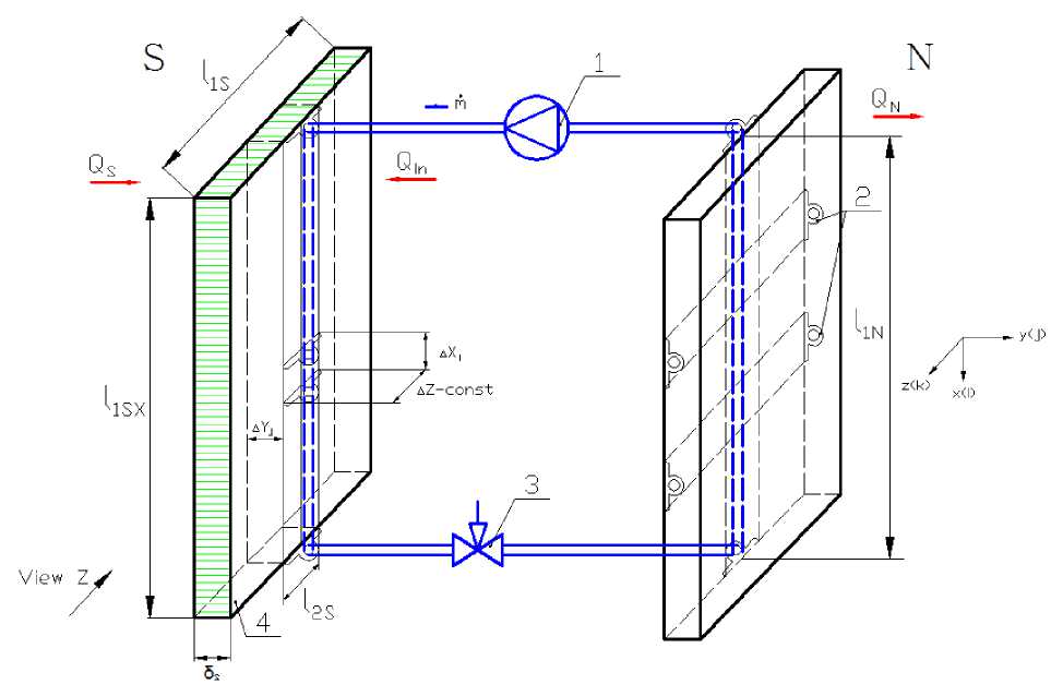
Fig. 1. Calculated two-dimensional thermal model of the thermal control system: 1 – compressor; 2 – heat pipes; 3 – throttle valve; 4 – honeycomb panel

Рис. 1. Расчетная двухмерная тепловая модель СТР:

1 – компрессор; 2 – тепловые трубы; 3 – дроссельный вентиль; 4 – сотопанель

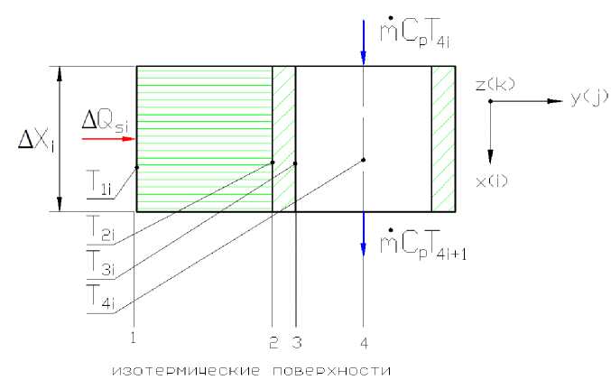
Fig. 2. Isothermal surfaces for the southern honeycomb panel

Рис. 2. Изотермические поверхности для южной сотопанели

Consider the process of two-dimensional complex heat transfer in the form of heat balance balance from the southern panel ( Q_S ), internal heat sources ( Q _int ) and heat release from the northern panel ( Q N ). The balance is a particular case of the energy conservation equation

Q s + Q int = Q n , (1)

where Q S is the heat flux passing successively through the isothermal surfaces of the southern panel (fig. 2): 1 – the outer surface of the southern panel with the temperature T 1 ; 2 – inner surface of the southern honeycomb panel with temperature T ₂; 3 – conditional inner surface of the liquid circuit with temperature T ₃; 4 – the surface along the average cross-section of the channel of the liquid circuit with the refrigerant temperature T ₄.

It is obvious that the heat flux Q_S , passing through the surfaces 1–2–3, is accumulated by the mass flow of the liquid circuit, in series (integrally) along the contact length l 1 S of the liquid contour of the southern panel. It should be noted that surfaces 1–2–3–4 are formed constructively by various boundary surfaces, thermodynamic properties of materials and types of heat transfer. In addition, the temperatures T ₁ –T ₄ are indicative values, that is, necessary for comparison with the maximum permissible values. For example, the temperature of the refrigerant T ₄ is necessary to evaluate the cavity supply of the liquid circuit.

Mathematical model . In the finite-difference form, the heat transfer at the i -th section of the southern panel (fig. 2) is determined by the following system of process equations [8]:

1. The heat flux from the Sun enters the surface 1 of the panel S:

(+) As ■ S0 ■AF ■ sin a, where AS is the absorption coefficient of solar radiation; S0 – solar constant, W / m2; F12 is the area of the radiation surface; α is the angle between the normal of the radiation surface and the direction to the sun.

This is emitted back into the open space [8]: ( ,^ A F T.

where ε₁ is the degree of blackness of radiation from the radiation surface; σ 0 = 5.67 ∙ 10^–8 – radiation constant, W / m^grad⁴; F ₁₂ is the area of the radiation surface, m²; T 1 is the temperature of the radiation surface, K.

The heat flow is diverted inside the honeycomb panel by heat conduction:

(-)

X 12 A F 12, " 12 ,

( T," T) ,

where λ12 is the thermal conductivity of the honeycomb material; δ12 – distance between surfaces 1–2.

The heat balance for surface 1 will be written as [9]:

AS ■ S0 ■ AF1i ■ sina — £1°0F12T —

'"^ F ( T i - T 2 i ) = 0,                ⁽²⁾

⁵ 12 i

formally, the heat flux at the surface element Δ F 12 i is determined like this:

AQi = as ■Sо ■ AF1i ■sina - £1^0F12T =

_ ^12 ^{A F} 12 i                             ⁽³⁾

X         ^{( T}1i    ^T2i ⁾ ■

° 12 i

2. The heat flux from the honeycomb panel is fed to the isothermal surface 2 by heat conduction

( + ) ^^A F ^ ^ ( Тц- T 2i ),

" 12 i

and is also taken away by the thermal conductivity to the inner surface (3) (fig. 2) of the liquid circuit

(-)

^ 23 ^{A F}23 i

23 i

( T 2 i - T 3 , ) ,

where λ23 is the thermal conductivity of the honeycomb material; δ23 is the distance between surfaces 2–3.

The heat balance for surface 2 is expressed by the equation

\A F ( T u - T)

° 12 i

^2^ ( T _M- T ₃ i ) = 0. (4) ° 23 i

3. The heat-conducting heat flux considered in (4) is fed to the surface 3

W^F3- (T2i-у, 5 23 i and the convective heat flow is already diverted into the liquid circuit

(-H^i' (T3i- T4i), where αi is the heat transfer coefficient.

The equation of balance over the surface 3 takes the form

^{Л A} F ( T 2i — Т з , ) — a _l ^ F з_{4 l} ( T 3 , - T i ) = 0.   (5)

⁵ 23 i

We group the equations of balances on surfaces 1–2–3 into the system:

A s ■ S 0 ■ A F ■ sin a - ^0 F 12 T 1⁴ -

-

^ 12 ^{A F}12 i

X^A F i 1 ° 12 i

^ 23 ^ F 23 i

⁵ 23 i

° 12 i

( T ii - T^

( T ii - T 2 i) = 0,

-

^л A F  ( TVT 3 i ) = 0,

⁵ 23 i

( T 2 i - T зJ-a , A F з4 , ( T 3 i - T 4 ) = 0.

It should be noted that (6) at a known coolant temperature at the -th element T ₄ is completely determined by the number of unknown variables – T ₁ , T ₂ , T ₃ , the system (6) is the basis of the marching algorithm when integrating along the length of the liquid contour of the southern panel [10]:

i = 4 Q s = £ a q_Sy i = 0

The temperature change T _{1 i} , T _{2 i} , T _{3 i} , T _{4 i} forms the projection of the temperature gradient on the transverse y ( j ) axis (fig. 2). The projection of the temperature gradient on the longitudinal axis x ( i ) is formed by the balance of the thermal power received during the heat transfer through the lateral surface (3) of the elementary calculated i -volume (fig. 2) and the difference in the thermal power of the refrigerant flow through the cross-sections at the output and input of the liquid circuit elementary calculated volume in step Δ X i :

A Q s, = mC p ( T 4i - T_4l+ i ) ,              (7)

Given T 40 – at the entrance to the liquid contour of the southern panel, given the values of thermophysical, geometric and regime determining parameters at the integration step, we calculate the system (6), (7) with respect to the unknown temperatures T _{1 i} , T _{2 i} , T _{3 i} , T _{4 i} , along the x ( i ) (fig. 1) at the length of the thermal contact of the liquid line with the honeycomb panel l_iS . Obviously, the integral heat output from the southern panel, including radiation and internal heat sources, is determined from an expression similar to (7) with regard to (1)

Q z S = Q s + Q int S = m t C p ■ ( T 4 n - T 40 ),               (8)

where T 40 is the temperature of the refrigerant at the inlet, and T 4 n is the temperature of the refrigerant at the outlet of the liquid circuit, Q _{int S} = Q _int is the heat from the internal sources supplied to the liquid circuit along the length of the thermal contact l iS (fig. 1) from the southern panel side, Q S is the radiation component of the heat input. It should be noted that heat from internal sources of Q _{int S} is physically formed from two components:

where Q int.fr is the frictional loss in the liquid circuit, turning into the heat of the coolant; Q int.HP is the zonal thermal power transmitted by the heat pipe from the working devices of the spacecraft. The temperature of the heat pipe, the area of the contact zone and its coordinates along the length l S are to be determined in the calculation scheme [11] (position 2 in fig. 1)

Let us consider the zonal heat input from the spacecraft through the heat pipe contact calculation case.

We assume that, as in the case of the radiation constant, the zonal thermal power is given and uniformly distributed over the contact area of the heat pipe at the finite length of the liquid loop Δ l iS = Δ l HP [12], then the input thermal power at the integration step is defined as: Δ q HP ∙ Δ F 65 . Let us pay attention that in the design scheme additional isothermal surfaces modeling heat transfer in a zone of contact of a heat pipe are entered: surfaces 6 and 5 (fig. 3).

Accordingly the system is supplemented with two equations:

q HP ■A F 6_{5 l}-^ ⁶5 ^{A F}5- ■ ( T 6 i - T ₅ i ) = 0;

° 65 i

^6^ ■ ( T 6 i - T 5 i ) - x . A F 54i- ( T 5i - T 4 i ) = 0.    (10)

⁵ 65 i

where m ɺ is the mass flow rate of the coolant in the liquid circuit, and C_p is the heat capacity.

In this case, the temperature at the entrance to the next calculated volume will be determined as

T = AQSi-4_T

T4i +1      .       ⁺ T 4 i '

mCp

The system ((6) and (10)) is completely determined by the number of unknowns. The zonal internal heat flux at the integration step is determined by one of the terms (10), for example:

AQintHPi = XiAF54i . (T5i - T4i) = ^^i- ■ (T6i - T5i) 565i or

⁵ 65 i

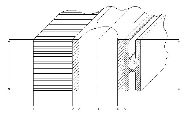
Fig. 3. Zonal heat input from the spacecraft through the heat pipe contact calculation case

Рис. 3. Расчетный случай с учетом зонального теплопритока от приборов КА через контакт тепловой трубы

The heat influx from internal friction at the integration step is equivalent to frictional losses [13]:

d _i    2

where λ f _r is the coefficient of hydraulic friction; Δ x_i is the integration step; d_i is the hydraulic diameter; ϑ _av is the average flow refrigerant velocity in the liquid path; m ɺ is the mass flow.

Taking into account (3), (11), (12), the total heat flux at the integration step is written as

Then, as in the case of a simple radiation heat load (13) from the balance of thermal power

∆ Q i Σ = m ɺ C p ⋅ ( T 4 i - T 4 i + 1 )             (14)

the temperature at the entrance to the next calculated (elementary) volume is determined by

∆ Q_{i Σ}

^{∆ T} 4 i + 1 ^{=       + T} 4 i ^.

mCp

Taking into account the fact that the temperature along the perimeter of the cross-section of the inner surface of the channel of the liquid circuit is a mean-integral value [14], the last equation in (10) is replaced by T3i = T5i, then the record (10) becomes simpler qHP⋅∆F65i-λ65∆F65i⋅(T6i-T5i)=0;

T 3 i = T 5 i                       (15)

Taking into account all the above-mentioned notations (1...15), we finally write down the heat balance equation for the southern panel:

A_S ⋅ S ₀ ∆ F ₁₂sin α -ε⋅σ⋅∆ F _{12 i} ⋅ T _{1 i} ⁴ - ^{λ 12 ∆ F 12 i} (T_{1 i} - T_{2 i} ) = 0; ^δ 12 i

^λ 12 ^{∆ F} 12 i _{(T 1 i - T 2 i )} ^δ 12 i

-

^{λ 23 ∆ F 23 i} (T 2 i - T 3 i ) = 0;

^δ 23 i

^{λ 23 ∆ F 23 i} (T 2 i - T 3 i ) -α i ∆ F 34 i (T 3 i - T 4 i ) = 0; ^δ 23 i

Т =т

^T3 i ^{= T}5 i ^;

q ⋅∆ F -λ ∆ F (T - T ) = 0;

TT 65i 65 65i 6i5

∆ Q = As ⋅ S ∆ F sin α-ε⋅σ⋅ ∆ F ⋅ T ⁴ =

Si                   0 1i1

^λ 12 ^{∆ F} 12 i

(T_{1 i} - T_{2 i} );

^δ 12 i

^δ 65 i

∆ x_i ϑ ² _av

d_i 2

∆ Q i Σ = m ɺ C p ⋅ ( T 4 i - T 4 i + 1 )

^{Δ Q} _{Σ S} ^{= Q}S ^{+ Q} int.S ^{= m ɺ C}p ( ^T 4 Sn ^{- T} 4 S 0 ) ^.

With the known determining parameters and thermophysical properties of materials, the set of equations (16) allows numerical integration over the length l_1S of the thermal contact of the liquid contour of the southern panel with the final result Δ Q_ΣS (8) and temperature field T _i j technically accessible for the measurement.

For the northern panel, we will retain all the methodological approaches and designations associated with constructive (isothermal) surfaces: T 1 is the temperature on the outer surface of the honeycomb panel; T 2 is one on the inside, etc. Solar radiation decreases (in our calculation case it is reset). Integration is conducted in the direction of the average flow rate along the thermal contact line of the liquid contour Δ l 1 N from the side of the north panel. We perform the necessary inversion of the signs and the specified additions we transform (16) into the thermal energy complex of the heat balance on the north panel:

-ε⋅σ⋅∆ F ⋅ T ⁴ + ^{λ 12 ∆ F 12 i} ( T - T ) = 0;

12 i 1 i                           2 i       1 i

^δ 12 i

-

^{λ 12 ∆ F 12 i} ( T 2 i - T 1 i ) +^{λ 23 ∆ F 23 i} ( T 3 i - T 2 i ) = 0; ^δ 12 i                         ^δ 23 i

-

^{λ 23 ∆ F 23 i} ( T 3 i - T 2 i ) -α i ∆ F 34 i ( T 4 i - T 3 i ) = 0;

δ23i т =т •

T₃ = T₅ ;

q ⋅∆ F -λ ∆ F (T - T ) = 0; TT 65 i 65 65 i 6 i     5 i

∆ Q Ni =ε⋅σ⋅∆ F 12 i ⋅ T 1 i ⁴ =^{λ 12 ∆ F 12 i} (T 2 i - T 1 i );

^δ 12 i

d_i  2

Q _{∑ Ni} = m ɺ C p ( T 4 i - T 4 i + 1 ) ;

^{Δ Q} _{Σ N} ^{= Q}N ^{+ Q} int.N ^{= m ɺ C}p ( ^T 4 N 0 ^{- T} 4 Nn ) ^.

It is necessary to pay attention to the fact that if external heat sources are insignificant, then on the northern panel there is an unambiguous decrease in temperature.

With the joint integration of heat and power balances ((16) and (17)), a mandatory condition

Δ Q _{Σ N} + Δ Q _{Σ S} = 0,            (18)

(see the last equations in (16) and (17)) is satisfied when the temperature differences are equal

Т — Т — т — т

T4Sn T4S0 = T4N0 T4Nn , or in another presentation – the temperature of the coolant at the output of the thermal contact of the liquid circuit of one panel basically determines the temperature at the input to the other:

T _{4 Sn} ≈ T _{4 N 0} ; T _{4 S 0} ≈ T _{4 Nn} , (19) clarification is possible with a specific topology of the hydraulic circuit of the liquid circuit outside the thermal contact lengths on the panels and hydraulic losses in the electric pump unit and the control throttle (fig. 1) [15].

Conclusion. The considered system of thermal balances of the thermal control system of the spacecraft on the characteristic surfaces of constant temperatures is reduced to the form allowing to conduct a numerical solution: the number of equations corresponds to the number of detected temperatures along the north and south panels and is closed through the coolant temperature of the liquid circuit. The system of equations makes it possible to investigate the thermal state of the spacecraft of a leaky design in the stage of preliminary design with varying mode (the angle of inclination of the radiation surfaces to the sun, the heat release of the service module and the payload module, etc.) and the design parameters (the specific dimensional topology of the object, diameter of pipe cross-sections, refrigerant flow, etc.), in order to deter- mine the area of efficiency and the area of optimum performance under certain performance criteria (for example: the ratio of mass of the thermal control system to power of diverted heat flow).