Using moving variance method to detect ocean currents from space

Currents in the ocean can be observed using indirect signs. It can be changes of sea surface temperature (SST) or phytoplankton. Another name for such signs is tracer agents. Tracer agents can be detected by passive sensors in visible and infrared thermal channels. These tracers visualize ocean currents in visible and infrared bands.

The NASA’s Sea-viewing Wide Field-of-view Sensor (SeaWiFS), Advanced Very High Resolution Radiometer (AVHRR) and Moderate Resolution Imaging Spectroradiometer (MODIS) provide images of such tracers. In order to detect ocean structure we should firstly understand the structure of phytoplankton and SST fields.

In seminal worldwide survey of oceanic fronts, Legeskis (1978) demonstrated a variety of SST fronts formed by vastly different physical processes. Shevyrnogov et al. have developed the special scientific program named “Chlorophyll in the bioshpere” and clearly shown the relation between dynamics of phytoplankton and large- and small-scale hydrological structure of the ocean.

• * Corresponding author E-mail address: artymail@mail.ru

  Based on mathematical model Kartushinsky (2004) estimated the spatial and temporal ranges of the SST frontal zones variation affected by the advection of currents, horizontal turbulent heat exchange, and the radiation heat flow in separate parts of the ocean.

2.    Methods and data

It is necessary to develop the image processing tool based on statistical treatment for allocation of oceanic structures. C.A. Brown et al. [3] uses clustering and principal component analysis to define the relationship between chlorophyll and ocean color. A. Turiel et al. [4] shown that the use of advanced image processing tools as wavelet singularity analysis allows to characterize the oceanic circulation patterns. Using statistical EOF analysis is it possible to explain the general seasonal cycle and quantify interannual variability of chlorophyll-a [5].

In a manner analogous to method of Shevyrnogov et al., 1996 we use a “moving variance” statistical method to reveal global ocean structure features [6]. Moving variance or quasistationary areas method is based on the statistical treatment of seasonal composites of satellite imagery. Quasistationary areas it is areas with the same type of seasonal dynamics. It means that change of parameter (chl-a or sst) in these areas occur equally.

The basis of the given approach is made by a box which moves on images and applies the following algorithm.

Let A k i j = { a_mn | m = i - q , i + q , n = j - q, j + q } is a set of pixels in a square with centre ( i, j ) for each season K . D k,i,j is a standard deviation for A k,i,j . Moving variance V i,j at the point ( i , j ) is a mean for D 1,i,j , D 2,i,j , D 3,i,j , D 4,i,j . For those areas where values change slowly values of moving variance are insignificant but it sharply increases where seasonal dynamics varies. Depending on parameters of a box areas with various spatial scales are allocated.

Shevyrnogov et al. [7] have shown that quasistationary areas can be a basis for the characteristic of fundamental biological and hydrological processes in the ocean. It can be a basis for definition of long-term trends of biological efficiency in the ocean. The continuous control of quasistationary areas reveals abnormal conditions of oceanic ecosystems.

Nine years of SeaWiFS satellite data from 1997-2005 were used to produce seasonal means and standard deviation estimates of chlorophyll-a concentrations for the global ocean. Seven years of MODIS imagery for 2002-2008 and twenty one years of AVHRR imagery for 1981-2001 were used to produce seasonal means and standard deviations of sea surface temperature for the global ocean. These images were downloaded from NASA’s ocean color website.

Statistical techniques for data mining are designed to extract useful information from large datasets and include methods such as moving mean, moving variance, smoothing of input and output data. Special software was developed using IDL (interactive data language). As a result more than 100 images has been obtained and analyzed.

3.    Results and discussion

The first set of data we used was chlorophyll-a distribution imagery. The results are shown in Fig. 1.

Dark areas correspond to the lowest values of variance, light areas it is areas with high variability and instability of phytopigment concentrations during one year.

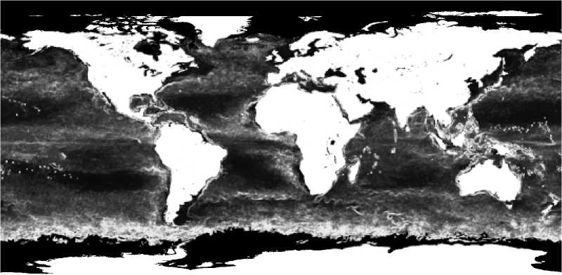
Fig.1. Areas with the same type of seasonal dynamics (QSA) from 264th day of 1997 till 263rd day of 1998

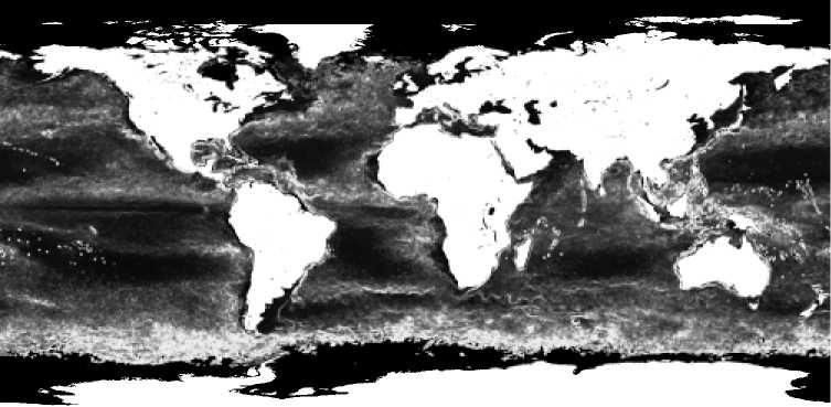
Fig. 2. Areas with the same type of seasonal dynamics (QSA) from 264th day of 2006 till 263rd day of 2007

Fig.1 shows the end of summer and the beginning of autumn. Almost the same picture we can see after nine years (Fig. 2).

These two images (Fig.1 and Fig.2) accurately allocate ocean structure. For instance, the map of QSAs in the Atlantic and the Pacific Oceans clearly shows the boundaries of the shelf waters at the western and the eastern coasts of the USA.

The next portion of data is satellite images of sea surface temperature. The results are shown in Fig. 3.

Here we have another type of colouring. Dark pixels corresponds to the high instability areas and light pixels belongs to areas with low variability of sea surface temperature.

Changing the size of a box it is possible to allocate structures of various scales. The smaller size of a box gives more detailed picture however brings more noise in the image. Nevertheless, the big size

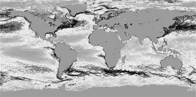
Fig. 3. Areas with the same type of seasonal dynamics (QSA) from 172nd day of 2002 till 171st day of 2003

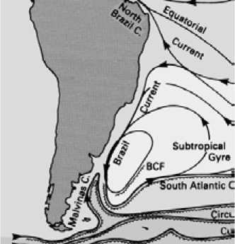
Fig. 4. Schematically image of Brazil Current of a box smoothes border of oceanic structures, the smaller box accurately allocates it. The results are shown in Fig. 4 and Fig. 5a, 5b.

4.    Summary and conclusion

Method of ocean structure revealing was developed. This method is based on detecting of quasistationary areas using “moving variance” algorithm. We have improved this algorithm to detecting areas with different spatial scales.

More than 1000 images have been processed. The ocean structure has been allocated using images of chlorophyll concentration and sea surface temperature [8].

Seasonal dynamics of chlorophyll concentrations and sea surface temperature in the ocean is one of the key factors indicating the types and intensity of hydrobiological exchange processes in the ocean surface layer [9].

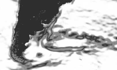
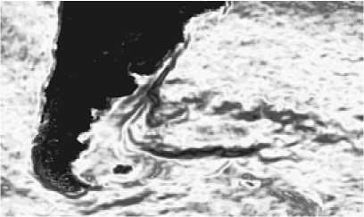
Fig. 5b. Brazil Current after QSA treatment (2003, 11x11 pixel box)

Fig. 5a. Brazil Current after QSA treatment (2003, 21x21 pixel box)

By focusing on the seasonal dynamics, we developed a useful observational tool for characterizing the type of dynamics.

Ocean structure revealed with the help of “moving variance” algorithm may form the grounds to characterize the fundamental processes of ocean biology and hydrology and helps to determine longterm trends of biological productivity in the global ocean. It also can help to check a hypothesis of global thermohaline circulation by detecting a global path of heat-and-mass transfer in the ocean.