Utilizing GVF Active Contours for Real-Time Object Tracking

Published Online May 2015 in MECS DOI: 10.5815/ijigsp.2015.06.08

Active contours or snakes have been widely used in many applications of image processing and computer vision. Ever since the introduction of the active contours by Kass et al [1], active contour models have received wide popularity with the computer vision community. It quickly found use in the different kinds of images or videos with applications such as image segmentation[2], image tracking [3][4], and object detection[5] [6].

In general, there are two different implement methods of active contours: parametric active contours[7]-[5], and geometric active contours (or geodesic active contours) [8][9].

Parametric active contours represent curves and surfaces explicitly in their parametric forms during deformation. This representation allows direct interaction with the model and can lead to a compact representation for fast real- time implementation. Adaptation of the model topology, however, such as splitting or merging parts during the deformation, can be difficult using parametric models. Geometric deformable models, on the other hand, can handle topological changes naturally. These models represent curves and surfaces implicitly as a level set of a higher- dimensional scalar function.

Object tracking is one of the fundamental tasks in the image processing techniques. In the past two decades many researches has been conducted in this field and many methods and algorithms have been introduced. These methods can be summarized into three major groups:

• A.    Point Tracking

In this method objects are represented as points in consecutive frames and these points are related to each other based on previous object situation which can be in form of position and movement.

This method needs an external mechanism for object recognition in each frame. For a single object tracking, Kalman and particle filters [10], and for multi object tracking JPDAF(Joint Probabilistic Data Association Filter) and MHT(Multi Hypothesis Tracking) are some of methods that are widely used [11].

• B.    Kernel Tracking

Kernel mostly considers the shape and object appearances. For example, kernel can be rectangular or elliptical shape with a defined histogram. Objects are tracked in the frames with estimation of their kernel trajectory. These trajectories are defined in form of translation, rotation and scaling.

• C.    Silhouette Tracking

Tracking is accomplished by estimating the object boundaries in each frame. Silhouette tracking uses the encoded information inside the object boundaries. This information can be in form of appearance density and shape models which are mostly edge maps. If the shape model in known Silhouette of object can be tracked using the image matching or contour evolution.

This method is used when articulated objects such as human body, hand, face are to be tracked.

In the contour tracking method, first an initial contour is selected, and then this contour is evolved in each frame until it reaches to the position of object in current frame. In this method, the object motion must be in a manner that the object boundary in the current frame overlaps with the previous and following frames. There are two methods that are commonly used to evolve the contour:

• -    using state space

• -    minimizing the energy function

In this paper, the third method, i.e. the contour tracking was considered. In the following section, a brief background was presented. Section 3 discusses optical flow approach in order to extract the edges of moving objects. Gradient Vector Flow (GVF) Active Contour approach is presented in section 4. Experimental results and discussions are presented in section 5 and 6 respectively. Finally, section 7 is dedicated to evaluate the performance of proposed algorithm.

II.    Research Background

In this section a brief review for object tracking is presented. The methods proposed by the researchers are as follows:

• A.    Tissainayagam et al. Method

Tissainayagam et al [18]. tried to present a tracking system utilizing the MHT, segmentation with contour and point tracking. In the first part of this work, the image edges are extracted using the MHT method, and then the contours are evaluated from these edges. The extracted contours are then mixed together for recognizing the objects. In the second part of the work, tracking is obtained from the first frame using MHT and some desirable key feature points extracted from edges.

For validation the proposed method in each frame, the extracted key feature points are compared to the segmented image. If an acceptable numbers of points are on the boundary or inside the object, then the tracking is considered to be valid.

• B.    Cheng And Foo Method

Cheng et. al. [3], proposed the contour tracking for non-rigid objects with the complex backgrounds images. They used Kalman filter with some changes which has resulted in a new filter called “structural Kalman filter”. This new filter takes into account the relation between the different parts of the moving object. This is done to overcome the measurement uncertainties when the object is overlapped by some the object in the scene. In this method, the estimation of the next object position is also achieved.

• C.    Koschan et. al. Approach

Koschan et. al. [12], used the active shape models for the non-rigid object tracking and changed the model so that it can be used for color images.

• D.    Ning et. al.

In this work, [13], a tracking system which uses a model based on kinematics of human motion and uses image matching and Hierarchical searching methods was presented. They also used a divide and conquer method to reduce the search space which utilizes a skeleton like model of human body. Then, an algorithm is used to update the joint angels of the model. For error calculations, a pose estimation function using boundary and region information is presented. As an initial condition, the estimated first frame is compared with 6 pre defined poses and the one which lies with the least error, was selected as the initial condition.

• E.    Kim et. al. Approach

Kim et. al. [14], tried to solve the active contour tracking short comings such as problems with intensity changes, object edge deformation, existence of other edges (complex back ground), and the edge noises in image with a system based on active shape models. Since active shape model is used, counters relations in different frames has been improved in comparison with the traditional active contour model.

• F.    Razi And Azadi Method

Razi and Azadi, [15], presented a novel algorithm for moving object detection which is based on GVF active contours. The method proposed in their work improves the GVF contour so the contour reaches the image edges in some concavities that the original GVF could not reach. This paper implements this method as a base for tracking system.

In the next section, the optical flow method is presented.

III.    Optical Flow

The main objective in optical flow method is to estimate velocity of pixels using temporal intensity changes in the sequence of images [16, 17].

One of the common assumptions for starting the work is that the intensity just moves from in successive frames:

I ( x , t ) = I ( x + u , t + 1)                q^

where I ( x , t ) is image intensity as a function of position vector x = ( x , y ) T and time. u = (u_x,u ₂) is the 2D velocity vector.

It should be noted that the above assumption is rarely satisfied and the real assumption is that the radiance of object surface is constant in successive frames (for example there are no mirror surfaces in the scene, the light source is a point which is far away so movements of the source does not have any effects on scene. Also the object is not rotating and there are no another reflections in scene). Although these conditions seem to be unreal, the equation works fine in practice.

Now let’s assume that the intensity equation can be estimated with Taylor series as:

I ( x + u , t + 1) = I ( x , t ) + u . V I ( x , t ) + I_t ( x , t ) + HOT . ^

Where V I = ( I_x , I ) and 1₁ are spatial and temporal derivatives of image intensity I and H.O.T. stands for the higher order terms of Taylor series.

If we neglect the higher order terms and substitute equation 2 into equation 1, we obtain:

M =

' Z gI 2    Z gI x I y'

5 x gI , I y   Z gI,²

V x            x      7

M has a rank of 2 and estimated velocity is calculated from the equation below:

и = M b

Using the resulted estimation, we can set a constraint to find the moving object:

V I ( x , t ) u + I_t ( x , t ) = 0                  (3)

| u 1 | + | u 2 | < T

The above equation relates the velocity to the timespace derivatives and is commonly known as gradient constraint. The resulted velocity vector u is known as image velocity or the optical flow. If only two frames are accessible or temporal derivative of image intensity cannot be calculated, a new gradient constraint can be achieved by substituting I with:

5 I_t ( x , t ) = I_t ( x , t + 1) - I_t ( x , t )             (4)

It is clear that equation 1 is not sufficient for estimating the velocities since two parameters of the speed are unknown. Gradient constraint just limits the velocity vector to a family of lines normal to V I with normal distance of I t     from the base. Since only

Л |V11|                                               J normal velocity can be calculated from equation (3), and there is no way to calculate tangent velocity, the complete velocity vector cannot be calculated (aperture problem). One way to overcome this problem is to assume that the velocity is the same in the neighbor pixels but there is a possibility that no velocity satisfy these constraints. Therefore, we would like to minimize the least square means of errors [19]:

E (u ) = Z g ( x ) U . V I ( x , t ) + ( x , t )] 2         (5)

x where g(x) is a weighting factor which is commonly assumed to have a Gaussian distribution. The velocity vector which minimizes the equation is assumed to be estimated velocity of image.

To calculate the minimum of the equation (5), the derivative of the equation is set to be zero. Thus we have:

5Е/Зи = Z8 (x )[u 1.Ix2 + u2IxIy + IxI* ] = 0

1 _x

5Е/зи =Eg(x )[u2.I" + u 1 IxIy + IxIt ] = 0

2x above equations can be written in matrix form:

Mu = b(7)

where the M and b are matrices as:

B

C

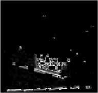
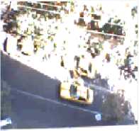
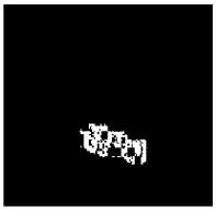
Fig. 1. a) original image, b) extracted edges which edges from previous frame is subtracted from it, the moving object after threshold.

pixels which satisfy the above constraint are considered to be the moving object and are subtracted from the edges of previous frame. Then the image is converted to a binary image using a threshold value.

• IV.    G radient V ector F low (G vf ) A ctive C ontour

Kass et. al. [1] introduced a new term called “Active Snake”. An active snake (contour) is a curve like:

X ( 5 ) = [ x ( ^ ), y ( 5 )], 5 e [0..1]               (11)

which tries to minimize the following energy function

E = ^ У₂( а | x '( 5 )|² +в | x "( 5 )| 2 ) + E ex. ( x ( $ ))] ds   ⁽¹²)

where α and β are curvature and hardness factors respectively. x ' , and x " are the first and second derivatives for X(s).

External energy term (Eext) is defined so that in the desired positions such as object boundaries, has the minimum value. Eext is commonly selected like this:

E e ⁽ x ¹ t ⁾ ( x , y ) =- | ∇ I ( x , y )| ²              (13)

E e ⁽ x ² t ⁾ ( x , y ) =- | ∇ ( G σ ( x , y ) ∗ I ( x , y )| ²         (14)

To extend the capture range of snake σ must have a high value, though this makes the edge of image blurry.

The snake which minimizes the energy function must satisfy the following Euler equation:

α x ′′ ( s ) - β x ′′′′ ( s ) - ∇ E_ext = 0            (15)

The above equation can be considered as an equation for equilibrium between two internal and external forces:

^F int ^{+ F}ext ^{= 0                      (16)}

For finding an answer to the above equation, both X(s) and parameter “s” are assumed to be time variable. Then, the temporal derivative of X(s,t) is set equal to the left side of equation (15). When the curve becomes stable the equation (15) is satisfied.

x_t ( s , t ) = α x ′′ ( s , t ) - β x ′′′′ ( s , t ) -∇ E_ext (17)

The method that Prince and Xu [20, 21] presented, introduces a new external force which is called “gradient vector flow” and is defined as:

Fex(tg)=v(x,y)

Substituting -∇ E  with this term leads to:

x (s,t) =αx ′′(s,t) -βx ′′′′(s,t) +v(19)

The curve that can satisfy the above equation is called a GVF snake. The gradient vector flow field is defined as:

V (x,y) =(u(x,y),v(x,y))

which minimizes the following function:

[ µ ( u_x ² + u _y ² + v _x ² + v _y ² )

^∫∫      + | ∇ f | ² | v -∇ f | ² ] dxdy

It can be proven that the equation (20) can be solved with the two following Euler equations:

µ ∇ ² u - ( u - f x )( f x ² + f y ² ) = 0           (22-1)

µ ∇ ² v - ( v - f x )( f x ² + f y ² ) = 0            (22-2)

where µ is a parameter which controls the dominance of the first and second terms of integral. These equations need a lot of calculations and processing resources which slows down the object tracking techniques. To solve this problem, different methods have been proposed [7-8].

One important problem that has a great effect on the system speed and contours convergence is the initial contour selection. In this paper, for initial contour selection, we selected some points over or near the edges of the object. Since the edges of moving object are extracted in the optical flow section, there is no need to calculate them. For reducing the time needed for calculation of GVF field and increasing the image processing speed, first a window containing the moving object and some pixels around it, is selected. Then the GVF field is calculated in this new window. In the following section, this results obtained based on our method is presented.

V.    Experimental Results

Experiments have been conducted in both indoor and outdoor environments. In both environments the system has an acceptable operation.

Methods and algorithms mentioned in the text are written in Code Gear RAD studio environment with DELPHI programming language. In all of the experiments, the threshold for converting the image to binary is set in a range from 50 to 120 (50 to 60 for low intensity, 70 to 90 for normal intensity and 120 for high intensity situations). Factor µ is set to be 0.2 in all experiments.

The developed software is tested on a laptop system with a core 2 due 2.55 GHz CPU and 4GB of RAM.

In the following section a brief discussion is presented.

VI.    Discussion

In our research work, we combine GVF tracking method with optical follow. Then, we demonstrated that the tracking has good speed. In fact, the GVF method provides good resolutions, while optical flow provides good speed for the tracking. Figures 2 to 8 shows the tracking pictures which are for different tacking situations. These situations were considered to examine tour algorithm. For instance, as shown in the figure 2, the track is for a situation where part of moving object was covered by another object. Also, in figure 3 tracking are done for a passing car in street. In our work, we assumed that there is only one moving object. Therefore, if another moving object appears in the scene, the tracker fails to track the objects. Figure 4 shows such a case where two moving cars are present in the scene.

Figures 5 to 8 shows the tracker performance in the indoor environment. Situations vary from low to high intensity which is from simple to complex backgrounds. Therefore, in all of the situations, the system is capable of tracking.

VII.    Conclusions

In this paper, a system is presented which utilizes the optical flow and GVF active contours methods for object tracking purposes. Active contours allow the user to have more details about object in comparison with other methods such as kernels or many other models.

Without code optimization, the system processes 10 to 12 images with size of 160x120 pixels which is good enough for many of object tracking.

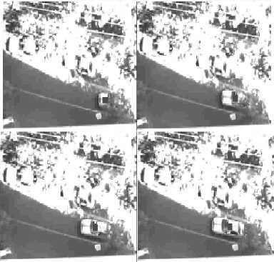
Fig. 2. - Tracking when the object is covered by another static object in the scene

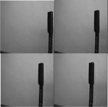
Fig. 5. - Tracking indoor with normal intensity and simple background

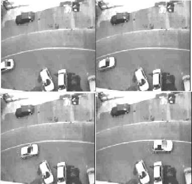
Fig. 3. - Tracking of a passing car in street

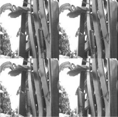
Fig. 6. - Tracking indoor with relatively high intensity and complex background

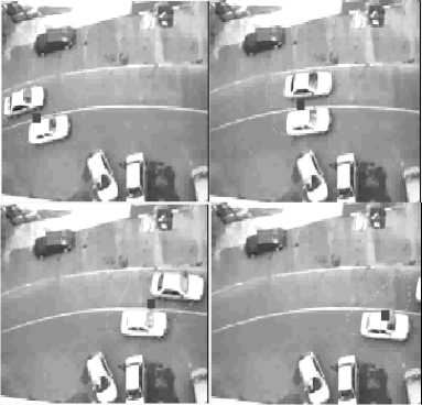
Fig. 4. - A case with two moving object. Due to the assumption in this paper the system fails to operate correctly

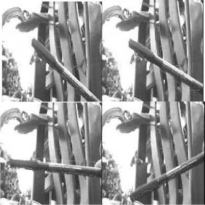
Fig. 7. -Tracking indoor. A Situation where the orientation of object changes.

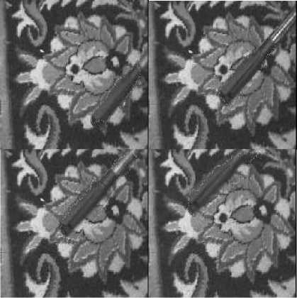
Fig. 8. - Tracking with relatively low intensity and complex background

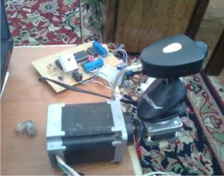
Fig. 9. - The implemented hardware for tracking