Узкополосное излучение с изменяющейся от 0.5 до 3.5 Гц частотой на фоне главной фазы магнитной бури 17 марта 2013 г

The frequency range 0.2–5 Hz of steady regular oscillations (Pc1 according to the classification of geomagnetic pulsations [Guglielmi, Troitskaya, 1973]) is represented in Earth’s magnetosphere by one of the main oscillation types whose structured subtype is most familiar as pearls. Other subtypes, frequency of which at least partially falls into this range, are ionospheric Alfvén resonator and serpentine emissions. However, the former are multiband and cover a wider range, up to 8 Hz [Polyushkina et al., 2015], whereas the latter ones are observed only in polar caps [Guglielmi, Dovbnya, 1973]. Both ground-based and satellite Pc1 observations show that besides structured pearls there often occur unstructured, usually narrowband, emissions in the same range. Either are said to be excited in the magnetosphere as ioncyclotron waves (ICW) due to kinetic instability of moderate energy (3–300 keV) ion fluxes [Cornwall, 1965]. The interest in Pc1 research is quite understandable considering the key role these pulsations play in solar-terrestrial relations [Guglielmi, Kangas, 2007]. They are sensitive to changes in dynamics and structure of the magnetosphere. These emissions have great diagnostic potential, providing insight into various magnetospheric processes as well as numerical estimates of key parameters of the medium [Gug-lielmi et al., 1972; Matveeva et al., 1972; Guglielmi, Troitskaya, 1973; Mursula et al., 1999]. This generally concerns the pearls observed under quiet and moderately disturbed conditions. There is, however, substantial interest in periods of strong magnetic disturbances with noticeable deformation and realignment of all structural formations in the magnetosphere. Below, we analyze a certain emission event, which occurred in the Pc1 range just against the background of a strong magnetospheric storm, which commenced on March 17, 2013 at 06 UT. This event is remarkable for its 9-hour duration and for extremely high nonstationarity of frequency varying during this event within nearly three octaves, from 0.5 to 3.5 Hz. The purpose of this study is to interpret the extraordinary event, comparing its properties with dynamics of disturbance development in the nightside magnetosphere. We hope that regularities revealed in this case study will provide further insight into phenomena leading to ICW generation during strong disturbances and into the relationship between oscillations excited and plasma processes in the magnetosphere.

OBSERVATIONS

On March 17, 2013, at 06 UT, Earth’s magnetosphere was attacked by an interplanetary shock front followed by a high-speed solar wind stream. Evolution of this disturbance can be traced from variations in the main geomagnetic indices and interplanetary electric field E (Figure 1). These and other data on conditions of the interplanetary electric and magnetic fields as well as geomagnetic indices were taken from the OMNI website [ ].

At 06 UT, the D st index sharply increased up to +15 nT. This indicates that the magnetosphere was compressed. At that moment, ground-based magnetic observatories registered a sudden storm commencement (SSC) followed by an increase in geomagnetic indices of auroral activity АЕ and planetary magnetic activity K р . The interplanetary electric field E abruptly strengthened later, at 08 UT. After the first positive pulse, D st began to decrease (this characterizes ring current development) and reached minimum at 20–21 UT, thus indicating the end of the main storm phase. Auroral activity peaked at 16 UT, and the global magnetic activity was maximum from 06 to 23 UT. The magnetic storm terminated by the end of the next day, on March 18.

During the first six hours of the storm, ultralow-frequency (ULF) oscillations behaved as usual for such conditions: abrupt pulses merging into a continuous irregular wave process in the form of PiB+PiC geomagnetic pulsations, which decayed by about 10:30 UT. However, at 12:30 UT, against PiB pulses some stations observed an emission band with an initial frequency of about 0.5 Hz and bandwidth 0.1–0.2 Hz (see Figure 2 that illustrates the dynamic spectrum of the emission in frequency–time coordinates as inferred from MND data; the observation interval is marked with vertical lines). The frequency gradually, for 30 minutes, increased from 0.5 to 0.7 Hz. Further there occurred an unusual stepped increase in frequency. First came the first step lasting for ~3 hours. Then, there was yet another frequency increase, and the next step formed. There were a total of three such transformations.

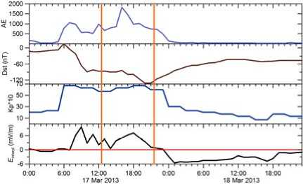
Figure 1 . Geomagnetic indices AE , D st , and K p , and interplanetary electric field Е (hourly average values) on

March 17–18, 2013. Vertical lines indicate the interval of observation of the emission at MND and UZR

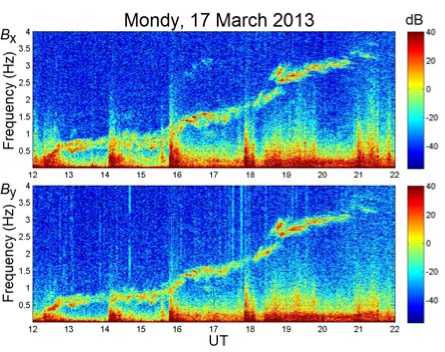
Figure 2 . Dynamic spectrum of two horizontal components of the variable magnetic field. The data were acquired from the output of induction magnetometer

Each transformation was not instantaneous – it took about 30 min. For 9 hr, the pulsation frequency increased approximately seven times, from 0.5 to 3.5 Hz. Each of these levels (steps) was not entirely horizontal, the frequency even in these steps increased smoothly; yet the emission band sometimes split, broadened to ~0.5 Hz, and individual structural elements in it became discernable. In general, the dynamic signal spectrum is very unusual and resembles a soaring dragon. The emission ended at 21:00–21:30 UT with a structural element of falling tone.

We managed to obtain data from induction magnetometers of seven stations located at different regions. Geographic coordinates of the stations, values of the McIlwain L parameter, and time difference (calculated by the model presented on the website [ gov/vitmo/]

for 2013 and for a height of 100 km) are set out in Table 1. The signal was observed only at three stations (Figure 3); the station Yakutsk (YAK) registered only the beginning of the signal, then it broke off. The stations Mondy (MND) and Uzur (UZR), spaced apart by 520 km, observed this signal almost simultaneously, its shape was nearly the same. YAK is 2100 km away from MND, but the available resolution of the record and the rather vague shape of the signal do not allow us to speak about any lag between observations of this emission at these two points. The station Borok (BOX), which is 3900 km away from MND, did not register even traces of the emission, neither did the other three stations, two of which (Dawson City (DAWS) and Thief River Falls (THRF)) are in the Western Hemisphere.

INTERPRETATION

It is widely agreed that Pc1 pulsations observed on the Earth surface reflect generation of ICW due to their interaction with energetic ions in magnetospheric plasma [Cornwall, 1965; Guglielmi, Troitskaya, 1973]. In general, however, the carrier frequency of emission remains constant or varies slightly. Here we deal with a sevenfold frequency increase. To understand the nature of the emission under study, we should answer the following questions: 1) Where are oscillations excited? 2) What is the cause for the abnormal frequency increase?

Let us discuss the well-known model of generation of ion-cyclotron emission in Earth’s magnetosphere [Cornwall, 1965]. It supposes that the instability that leads to ICW excitation arises from resonance of wave field with ion cyclotron motion in magnetized plasma at the frequency below the ioncyclotron frequency. To accomplish this, the phase velocity of wave, which may be considered equal to the Alfvén velocity А , should be lower than the longitudinal component of ion thermal velocity W ||i , i.e., W ||i >> A . In this case, the frequency f w of generated ICW is

f = A 5t J w W№ 2n ’

where

^A = Bl^{4 П} m P ^N ieff and ^N ief = ^N P I ¹ + E m - ^N i Im P ^N P I . \ i

Here Ω i = e i B / m i c is the ion gyrofrequency; e i and m i are the ion charge and mass respectively; N p is the proton density, the summation in (1) is performed over all types of ions except protons; В is the magnetic field; с is the velocity of light. The condition W ||i >> A and Formula (1) impose certain constraints on the region of wave excitation and ion energy generating oscillations of a given frequency. Let us consider them.

Turning from the thermal velocity W||i to the longitudinal proton energy E||i, we rewrite (1) as follows f =

w

e _i

B ²

^{4 n} m i c J2 П N ieff Ei ’

or, substituting values of physical constants and expressing the magnetic field in nT, density in cm–3, and energy in keV, we obtain the ICW frequency in Hz:

f =

w

7.6 - 10 " 4

_I2B₌ Г m p ) 7 N ieff E l m 1 J

where m p is the proton mass, k is the multiplicity of resonant ion charge. Then, we should determine conditions favorable for ICW generation within 0.5≤ f w ≤3.5 Hz. Substituting the observed frequency values in (3) yields a two-sided inequality

24 m

4.33 - 10 5 Гц ²< —----- 1 -p-|< 2.12 . 10 7 Гц ² .

N ieff E |1 l m 1 J

However, W ||i >> A in convenient units of measurement rearranges to the form

N ieff E ii m

^ >>  2.48 - 10 ^{- 3} .

B ²

m _i

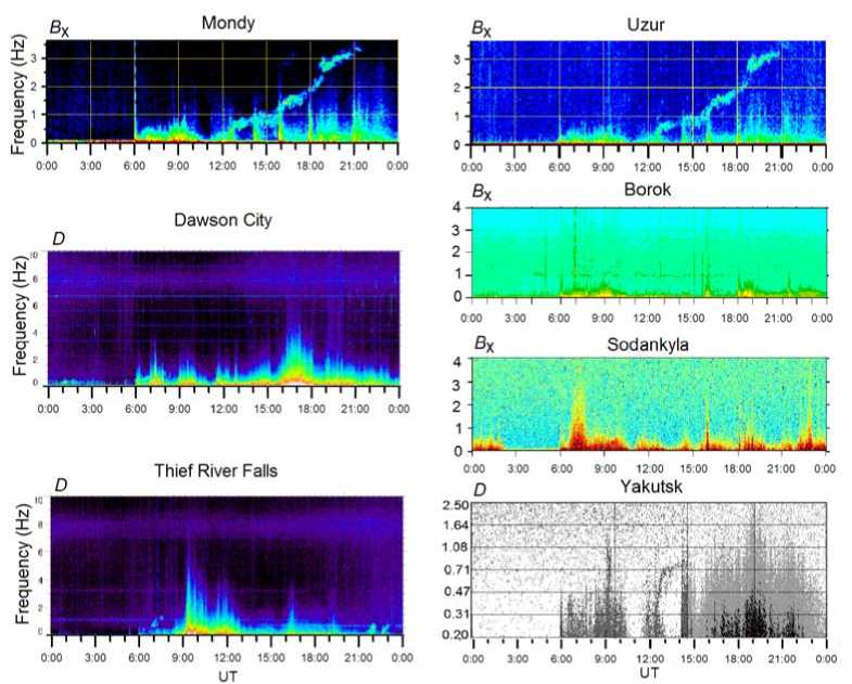
Figure 3 . Spectrograms constructed from records of induction magnetometers for March 17, 2013. Letters denote magnetic field components used for obtaining dynamic spectra

Next, we determine which plausible values of plasma energy and density can satisfy this inequality in the magnetosphere.

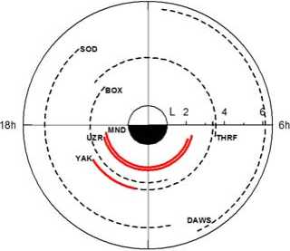
But first let us give the general picture of observation of Pc1 pulsations at different ground-based stations. Figure 4 shows trajectories of seven stations in polar coordinates (the view from the North Pole, the Sun is at the top), which are equipped with the induction magnetometers data from which we analyze 20

(Table 1). As has been said above, the signal of interest was detected only at three stations; at YAK it was observed only for the first three hours, then it disappeared.

Table 1

Station	Geographic coordinates		L parameter	Local time at midnight GMT
	φ	λ
Dawson City (DAWS)	64.0	220.9	6.1	10.3
Sodankylä (SOD)	67.4	26.6	5.4	21.2
Thief River Falls (THRF)	48.0	263.6	3.5	6.6
Yakutsk (YAK)	62.0	129.7	3.4	15.8
Borok (BOX)	58.1	38.2	3.0	20.8
Uzur (UZR)	53.3	107.7	2.35	16.9
Mondy (MND)	51.6	100.9	2.2	17.3

The most probable region of pearl generation is usually thought to be the plasmapause and its adjacent plasmaspheric regions [Glangeaud, Lacoume, 1971; Guglielmi, Troitskaya, 1973; Mazur, Potapov, 1983]. This is also confirmed by direct measurements of ICW onboard Cluster satellites [Pickett et al., 2010]. Ring current ions cross regions with higher plasma density, thus ensuring fulfillment of (5). In disturbed conditions, the plasmasphere suffers erosion under the action of the electric field penetrating into the magnetosphere, and the plasmapause is situated on the magnetic shells L _p<4. The event we consider occurred during the main phase of the strong magnetic storm when the D st index representing ring current intensity decreased below –130 nT.

12h

Oh

Figure 4 . Diurnal trajectories of the seven stations, equipped with induction magnetometers, in polar coordinates (the view from the North Pole, the Sun is at the top). The origin of each trajectory shown by a dashed (or red) line corresponds to 12 UT, each with the respective station code. The trajectory sections in which the signal was registered at the corresponding station are indicated by red lines

Unfortunately, we cannot precisely localize the plasmapause during observation of the signal because satellites capable of measuring its position when crossing plasmasphere boundary (Cluster, Themis) were in other magnetospheric regions at that time. Numerous empirical models predicting the position of the plasmapause [Carpenter, Anderson, 1992; Moldwin et al., 2002; Liu et al., 2015; Cho et al., 2015;

Verbanac et al., 2015] work badly under high magnetic activity. It suffices to say that substituting real solar wind parameters and geomagnetic indices for March 17, 2013 in the model [Verbanac et al., 2015] gives negative L p values for night hours. Nevertheless, comparing dynamics of the magnetosphere during this storm with that during other magnetic storms, namely 22–23 April 2001 and 28–31 October 2003 ones [Goldstein et al., 2005; Liu et al., 2015], we can make quite reasonable assumptions about dynamics of the plasmapause during this event. So, in the course of the main phase of the weaker storm on April 22, 2001, the plasmapause in the night sector moved to L p =3 (Figure 2 in [Goldstein et al., 2005]). During the much stronger storm on October 28–31, 2003, the plasmasphere in the main storm phase shrank to such an extent that in the night sector the plasmapause took the position L p ≤2, although before the storm it was at L p =4 (see Figure 9 in [Liu et al., 2015]). It is fair to assume that in our intermediate case the plasmapause during the second half of the main storm phase could shift in the dusk-midnight sector from L p =3–4 to L _p=2.4–2.7. This assumption is also supported by the behavior of the geomagnetic indices in Figure 1, where the K _p and АЕ indices as well as the interplanetary electric field are shown to have had higher values several hours before the time interval 12–22 UT under study. This points to energy accumulation in the magnetosphere, which contributes to erosion of the plasmasphere.

However, the foregoing does not allow us to grasp the general picture of appearance, evolution, and observational conditions of the emission considered. Indeed, Figure 4 raises the following questions. First, why did the higher-latitude stations SOD and DAWS observe no emission, and why did the station BOX, which entered the dusk-midnight sector 4 hours after MND, not see even traces of the emission, while UZR and MND continued observing it? Second, why was the emission interrupted at YAK at about 23 LT? And, third, the key question. What produced the sevenfold increase in the emission frequency at MND and UZR? A possible explanation could be the assumption about the presence of a local source of pulsations at 50-55 ° N in the meridional interval 100-105 ° E, which rotates with Earth and hence is located somewhere at fairly low heights, in the plasmasphere or ionosphere. Such a source is described in [Yahnin et al., 2007; Ermakova et al., 2015]. Authors generally associate their observations with spot-like precipitations of protons or heavy ions [Bräysy et al., 1998; Søraas et al., 2013]. However, we think that such precipitations, which are largely local and short-term [Bräysy et al., 1998], cannot explain the longterm continuous emission observed on March 17, 2013. Below, we try to answer the questions, offering another explanation.

Figure 5 shows a spectrogram of the signal we analyze ( а ) in frequency–time coordinates and variations of the magnetic disturbance index at low latitudes SYM-D ( b ), auroral activity index АЕ ( c ), interplanetary electric field E y ( d ), vertical component of the interplanetary magnetic field (IMF B z , e ). In addition to the signal, we should pay attention to the vertical bursts at the bottom of the panel (Figure 5, a ). These are irregular PiB pulsations; they reflect instants of injection of charged particles into the ionosphere. During weak and moderate disturbances, the injections occur at auroral latitudes, but during strong magnetic storms they take place at middle latitudes. Therefore, in the figure, the instants of PiB occurrence almost do not correlate with AE variations, but they coincide well with enhancements of low-latitude magnetic disturbances ( SYM-D ). Besides, they all are seen to appear some time after the southward rotation of B _z, during periods of negative values of the IMF component when magnetic field lines 22

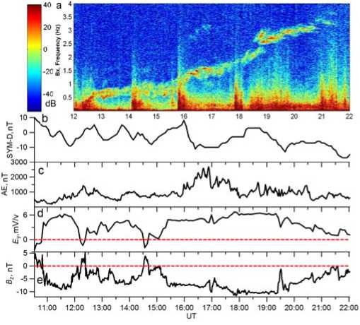
Figure 5 . Dynamic spectrum of the emission under study ( a ) and simultaneous variations of geomagnetic indices and parameters of the interplanetary electric and magnetic fields: the SYM-D index representing the symmetrical part of the azimuthal component of low-latitude geomagnetic disturbances ( b ), the auroral activity index АЕ ( c ), the Y component of the interplanetary electric field E y ( d ), the vertical IMF component B z ( e )

merge in the front of the magnetosphere. A comparison between the instants of PiB occurrence and the dynamic spectrum of the signal shows that the injection is followed by enhancement of attenuated signal (at about 14 UT), frequency increase (at ~ 18 UT), or by a combination of both (16 UT).

It is of interest that after 16 UT at the bottom of the spectrogram there arises another type of emission – geomagnetic PiC pulsations ("hisses"), which have the form of continuous darkening over the horizontal axis; and after 18 UT, PiC are superimposed by successive weak PiB pulses. All these suggest increasing wave activity in the magnetosphere.

As inferred from studies of dynamics of the magnetosphere during strong magnetic storms [Smith, Hoffman, 1974; Zhang et al., 2015; Dandouras et al., 2009; Goldstein et al., 2005], its interaction with the impact solar wind stream produces two key processes: 1) transfer of magnetic field lines from the dayside magnetosphere to the tail with subsequent reconnection in the neutral layer of the tail and injection of accelerated ions into the nightside magnetosphere with formation of nose-like structures of energy spectra corresponding to quasi-monochromatic fluxes; 2) penetration of the interplanetary electric field leading to an increase in the internal magnetospheric electric field dawn-dusk and hence to the enhancement of convection and gradient drift, which cause the plasmasphere to erode and the plasmapause to approach Earth. Both the processes occur in the pulse mode, being followed by precipitations of electrons and thermal ions into the ionosphere with generation of bursts of irregular PiB pulsations. Referring to Figure 5, we can assume that those PiB pulses which precede enhancement of emission intensity appear under the action of the negative IMF B z (Figure 5, e ) initiating process 1, whereas those pulses after which emission frequency increases are triggered by process 2 – the interplanetary electric field (Figure 5, d ) penetrating into the magnetosphere. Of course, both the processes are closely interconnected.

Let us reconstruct the sequence of events. Following the shock front, which reached the magnetopause at 06 UT, the magnetosphere was affected by a high-speed stream of interplanetary plasma. The solar wind dynamic pressure increased, the direction of the IMF B z component changed very rapidly, but its hourly average values were negative (Figure 5, e ). The influence of the high-speed stream on the geomagnetic field led to its disturbance, causing the magnetospheric storm. The ring current intensified greatly. This reflected in the behavior of the D st index: by 20 UT, it fell to –132 nT; the general level of magnetic activity went up: K p rose to 6.7, АЕ to 1822 nT (Figures 1, 5, c ).

Under such conditions, as is noted by the authors of [Goldstein et al., 2005] who studied the behavior of the magnetosphere during the above mentioned storm of April 22–23, 2001, each interval of the southward rotation of IMF B z is followed by dayside reconnection and, with a half-hourly delay by earthward motion of the plasmapause. Besides, the mutual action of the enhanced convection, gradient drift, and corotation leads to ion transfer from the plasma sheet to smaller L shells in the plasmasphere [Smith, Hoffman, 1974]. In this case, corotation and gradient drift give rise to the so-called nose-like structure in the dynamic ion spectrum; the front edge of the "nose" penetrates into the plasmasphere, it is represented by almost monochromatic 5–15 keV ion fluxes replenishing the ring current [Smith, Hoffman, 1974; Zolotukhina, Bondarenko,1976; Burke et al., 1998; Ganushkina et al., 2000]. In [Zolotukhina, 1982; Kangas et al., 1998], the authors show that in the vicinity of the nose, Cherenkov or cyclotron generation of Pc1 waves occurs respectively under isotropic or anisotropic particle distribution over pitch angles. In the case of reiterated successive injections caused by repeated impacts of southward IMF on the magnetosphere and also as the convection field increases, the energy of ions coming from the tail can rise several times [Zolotukhina, 1982; Kangas et al., 1998], exceeding at least 32 keV [Dandouras et al., 2009].

With this consideration in mind, we can propose the following sequence of further events as one of the possible variants. At 12 UT, against the background of energy input from the solar wind (starting at 06 UT), there arose ICW which propagated along field lines to the Earth surface and were observed as Pc1 geomagnetic pulsations at three stations: MND, UZR, and YAK (Figures 3, 4). The region of ICW generation must have been located at the outer boundary of the plasmasphere, immediately under the plasmapause. At 12 UT, the near-midnight part of the plasmapause was between 3.5 and 4 L shells. At the same time, the plasmasphere started to be affected by accelerated moderate-energy ions from the geomagnetic tail. Further, taking into account the conclusions drawn in [Goldstein et al., 2005; Dandouras et al., 2009; Liu et al., 2015; Cho et al., 2015], it is fair to assume that in subsequent hours, on the one hand, the plasmapause approached Earth and by 21 UT reached L p =2.5–3 in its near-midnight part; on the other hand, the successive injections produced particle fluxes of increasing energy, which penetrated deeper into the magnetosphere, reaching outer areas of the plasmasphere.

To understand how these processes affected conditions of generation and frequency of excited ICW, we estimate physical parameters of the medium in the assumed regions of wave generation, using the Tsyganenko magnetic field model [] and available direct satellite observations made during analogous geomagnetic disturbances. Thus, summarizing electron density measurements, reported in [Liu et al., 2015; Cho et al., 2015], we can conclude that during disturbed periods in the nightside plasmasphere the elec-24

tron density obeys the law N e -2 - 10 7 L ^-6. 7 cm^-3. Turning from this value to the effective ion concentration, which determines the Alfvén velocity (see (1)), we take into account that the plasmasphere, especially during disturbed periods, has admixtures of heavy oxygen and helium ions as much as 20–30 % of protons with respect to the number of ions per unit volume. This causes the effective plasma density to become equal to

, ,,      ,, 1 + 4ц + 16ц

P pl = m p k heavy N e = m p ^N e ---------- ,                                                               ⁽⁶⁾

1+ П + Ц where n=NHe+/Np; Ц=Nо+/Np. The coefficient kheavy under disturbed conditions in the plasmasphere can vary within kheavy=2-3, therefore for rough estimates we can set Nieff-5-107L-6.7 cm-3.

Let us trace magnetic field variations on the plasmapause from 12 UT when the main station observing the signal (MND (X-100°)) was at the meridian of 19 LT, and to 22 UT when it was already in the pre-dawn region, at the meridian of 05 LT. According to the Tsyganenko geomagnetic field model [], in the near-midnight region at L=3–4 the magnetic field between 12–14 UT on March 17, 2013 was from 360 to 1100 nT. Later, between 15-19 UT when the meridian X=100° moved to the midnight, the magnetic field on the plasmapause, which shifted toward Earth to L=2.8–3.4, was already 600–1350 nT. At the end of the event, at 20–21 UT, the plasmapause dropped to L=2.4–2.7, where the magnetic field was 1500–2100 nT.

According to the results obtained in [Smith, Hoffman, 1974; Dandouras et al., 2009], the energy of ions coming from the geomagnetic tail, as previously noted, could vary from 5 to 32 keV during the main storm phase. Summing up these estimates of the medium parameters, we can construct a scenario describing the connection between ICW frequency variations with evolution of the plasmasphere and resonant ion fluxes at a time when a magnetic storm develops. Such a scenario is illustrated in Table 2. The table is compiled in the assumption that the emission is generated in the form of ICW just below the plasmapause in the vicinity of the midnight meridian, and then the waves that fall on the ionosphere along field lines propagate along the ionospheric waveguide in azimuthal and equatorial directions. In Table 2, the whole period of the observed emission is divided into five time intervals, each with more or less stable oscillatory mode. The first two columns present the beginning and end of each interval in universal time

Table 2

Observed range of frequency variations, position of the plasmapause L p , and guess values of plasma density N ieff , magnetic field B p , resonant proton energy E res in the wave generation region just below the plasmapause at the midnight meridian

Time interval		f w , Hz	L p	N ieff , cm–3	B p , nT	E рез , keV
UT	LT MND
12:30–14:05	19:30–21:05	0.5–0.7	4.0–3.8	(4.6-6.5) - 103	360–445	8.4–7.1
14:05–15:45	21:05–22:45	0.5–1.2	3.8–3.35	(0.5-1.5) - 104	445–780	13.9–7.7
15:45–18:45	22:45–01:45	0.9–2.4	3.35–2.8	(1.5-5.0) - 104	625–1320	13.7–6.0
18:45–21:00	01:45–04:00	2.5–3.5	2.7–2.4	(6.4-14) - 104	1500–2070	7.3–6.1
21:00–21:30	04:00–05:30	3.5–3.2	2.4	1.4 - 10 5	2070–2040	6.1–6.9

(UT) and local time (LT) at MND. The third column gives the range of the observed frequencies f w for each time interval; the forth one, the range of changes in the plasmapause position L p ; the fifth, respective values of the effective background plasma ion density immediately under the plasmapause; the sixth, respective field values at the midnight meridian, which were calculated using the Tsyganenko model T01. The seventh column shows resonant proton energy values necessary for ICW generation under the above conditions in accordance with Formula (3). Condition (5) is confidently fulfilled everywhere.

The first interval is the beginning of oscillations, there is a small increase in frequency associated with a slight earthward shift of the plasmapause and the respective magnetic field enhancement. The resonant proton energy range is narrow, the energies themselves are also lower than moderate ones. The injection at the beginning of the second interval caused no increase in frequency, i.e. the plasmapause is likely to remain in its former place, L _p=3.8. However, emission intensity somewhat enhanced and frequency band broadened. This must have been associated with the ejection of new proton fluxes from the tail with wider energy spectrum, which included energies up to 14 keV. The emission frequency rose only by the end of the second interval. This is likely to be due to the weak pulse at 15:35 UT. It bears witness to strengthening of the dawn–dusk field in the magnetosphere, which can move the plasmapause inside by 0.45 R E within a very short space of time. The third, longest, interval is characterized by a steady frequency increase with a significant enhancement of oscillation intensity at the beginning of the interval. This may be explained by a new injection at 15:45 UT. Another increase in the rate of frequency rise with simultaneous intensity enhancement occurred after the double pulse around the 18 UT hour mark. The frequency increase was due to the magnetic field strengthening caused by significant compression of the plasmasphere (at 0.55 R E ). At 18:30 UT, the mode of injection into the magnetosphere changed. This is evidenced by the pattern of low-frequency pulses; their intensity decreased, and then they followed one another almost continuously. This might have resulted in the abrupt, nearly instantaneous shift of the generation region to lower heights, at least by 0.1 R E , as well as in the enhanced proton flux from the geomagnetic tail. In the end, during the last, fifth interval, the emission frequency went down for the first time. We think that during this 30-min period the plasmapause held its position, whereas the frequency decreased largely due to reduced magnetic field at the same height owing to the regular change of the field pattern in passing from the main storm phase to the recovery one, according to the Tsyganenko model T01. Finally, note that not only protons, but also helium and oxygen ions might have been resonant. Then, the particle energy required to generate emission of the same frequency should be 4 times lower for helium ions and 16 times lower for oxygen ions. But for oxygen, inequality (5) would not be strict any more, i.e. the thermal ion velocity would be only slightly higher than the Alfvén velocity.

Note also that in Formulas (1)–(5) the ion thermal velocity and energy are represented by their longitudinal components W || _i and E || _i. At the same time, the ion-cyclotron instability requires a fairly strong temperature anisotropy of the type T_n >  T to appear; therefore, in actual fact, values of total energy needed for ICW excitation (Table 2) should be higher.

Now we can answer the three questions posed above concerning the nature of the observed emission.

• 1.    ICW were excited by protons of moderate energies (5–14 keV) in the outer area of the plasmasphere, immediately under the plasmapause. Then, they propagated along field lines to the ionosphere, where they partially leaked into the Earth surface and partially were captured in the ionospheric waveguide. In the waveguide, the protons could move in the azimuthal direction and toward low latitudes. Poleward behind the projection of the plasmapause in the ionosphere there was a zone of strong turbulence with lower plasma density – ionospheric trough. Therefore, the waves could not propagate poleward. That is why they were not observed at stations located at higher latitudes than YAK.

• 2.    During the main storm phase, the plasmapause shifted to lower L shells associated with stations located at ever lower latitudes. At ~15 UT, YAK was outside the plasmasphere, in the ionospheric trough; therefore, the signal was interrupted there. The Thief River Falls station is located at nearly the same latitude as YAK, but during the emission generation it was in the dayside sector, therefore the signal was not observed there even at the first hours of the event.

• 3.    The main role in the frequency increase is played by the magnetic field strengthening in the generation region as the plasmapause approaches Earth. This is evident from Formula (3) in which the magnetic field B is raised to the second power, by contrast with plasma density and proton energy raised to the power of ½. The magnetic field varies depending on the position of a shell on average by the law B ~ L ^–3; hence the shift of the generation region by 1.6 R _E turned out to be sufficient for the sevenfold frequency increase, although plasma density rose thirty times then.

Note that the scenario of the described event we propose makes no pretense to completeness and is not the only possible. Nevertheless, we believe that it might well have occurred in reality.

DISCUSSION

The event considered is unique because such prolonged regular emissions in the range 0.2–5 Hz with such a wide range of frequency variation have not been observed before. In morphology the closest to the emissions of interest are Pc1 structured emissions ("pearls") with gradually varying frequency [Feygin et al., 2000] and irregular pulsations of diminishing periods (IPDP) [Sizova et al., 1977; Guglielmi, Zolotukhina, 1978]. However, pearls with varying carrier frequency usually last no more than 5–6 hr, although there are exceptions [Ermakov et al., 2015; Kim et al., 2016]. Most significantly, the range of variation in frequency of pearls is within 1.5 octaves (the ratio of the maximum frequency to the minimum one is less than 3). Besides, they occur at a lower level of magnetic activity. The events discussed in [Feygin et al., 2000] were registered at AE indices which were no higher than 600 nT, whereas in our case its hourly average value was as high as 1800 nT (Figure 1). Unlike pearls, IPDP can be seen during high magnetic activity in both the main and recovery storm phases [Sizova et al., 1977]. In this case, their generation is attributed to injections of charged particles from the tail into the inner magnetosphere [Gug-lielmi, Zolotukhina, 1978]. However, IPDP usually have the noise character, although discrete elements can sometimes break through the noise bandwidth [Guglielmi, Troitskaya, 1973]. Still, IPDP refer to irregular geomagnetic pulsations. They have a wide frequency band, instantaneous values ∆ f / f ≈1 with typical duration of the event ∆ t ≈20–100 min. The range of frequency variation is narrow, normally from 0.5 to 2 Hz. However, if we try by all means to put the observed phenomenon into any frames, the event under study can be considered the rarest case of long-term narrowband and extremely unsteady IPDP emission.

Ошибка оригинал

What unusual conditions inside and outside the magnetosphere could induce generation of such emission? First, it is a very long, ~16 hr (if we take hourly average values), period of negative values of the IMF B z component and thus of positive and high values of the E _y component of the interplanetary electric field. This stimulated the long process of iterative pulse injections of ions from the magnetotail. An important factor was the formation of nose-like structures in the space-energy spectrum of penetrating particles. This resulted in mono-chromatization of fluxes and thus in the generation of ion cyclotron waves with narrower bandwidth than in the case of ordinary IPDP. Concurrently with the injection, the interplanetary electric field penetrating into the magnetosphere triggered a fairly long process of plasmasphere erosion. This led to a steady, 8–9 hr, shift of the generation region to smaller L shells with a stronger magnetic field.

We hope that the proposed picture of occurrence of the unusual emission will help to clarify some additional details of processes occurring in the magnetosphere during strong disturbances caused by highspeed solar wind streams.

CONCLUSIONS

• 1.    We have presented the results of registration of a narrowband Pc1 emission of unusually long duration with increasing carrier frequency. The emission occurred during the main storm phase and was local, manifesting itself only at three stations located in the longitude range Z=100-130 ° Е and magnetic shells L =2.2–3.4.

• 2.    We have proposed an interpretation of the emission, which is based on the standard model of generation of ion cyclotron waves in the magnetosphere by ion fluxes of moderate energies. It is expected that the continuous shift of the ICW generation region to smaller L shells is able to explain both the local character of the phenomenon and the range of the frequency increase.

• 3.    We have formulated morphological differences between the emission and well-known types of geomagnetic pulsations and discussed reasons for the occurrence of this unusual event.

The work was supported by the Russian Foundation for Basic Research, grants No. 16-05-00631, 1605-00056, and 15-45-05108. We express gratitude to N.A Zolotukhina for her contribution to understanding of the problem, A.V. Guglielmi for discussion and valuable advice, B.I. Klain for his help in the study, and A.V. Moiseev for helpful comments. Interplanetary observations were taken from the GSFC/SPDF OMNIWeb website []. We grateful to Tero Raita (Sodankylä) [] and CARISMA I.R. project managers Mann and D.K. Milling [Mann et al., 2008; ], and to the project team (the Dawson City and Thief River Falls stations) for the on-line access to diurnal spectrograms of geomagnetic pulsations, and also to S.V. Anisimov and observers from the Geomagnetic Observatory Borok []. The magnetic field has been calculated by the on-line model T01, devised by N. Tsyganenko (SPSU), of the Community Coordinated Modeling Center situated at NASA Goddard Space Flight Center [].