Variable Structure Control on Active Suspension of 4 DOF Vehicle Model

Published Online December 2010 in MECS

Passive vehicle suspensions are based on a trade-off between conflicting requirements. Once designed, parameters of the passive suspension system can’t be changed and that limits the further improvement of the car’s performance. To obtain a high ride quality, active/semi-active suspensions were proposed. Active suspensions with energy supplied from outside can adjust the energy flow continually to accommodate the extensive external disturbance, which can meet the safety requirements as well as the comfort requirements. Controller strategy is the core of the active suspension design, for its validity and the data processing scheme determine the final performance of the active suspension system.

Variable Structure Control is a switching feedback control which provides a simple tool for coping with uncertain nonlinear plants. The computer technology and high-speed switching circuitry have made the implementation of VSC of increasing interest to control engineers. The control action is used in order to maintain the system state trajectory on a prescribed sliding surface. However, because of non-ideality of switching the problem of chattering arises, which constitutes a major limitation in real-world applications. Recently, research efforts have been made in order to offer modifications and extensions of the basic theory to alleviate this problem.

Variable structure model following control (VSMFC), based on the theory of variable structure system, which was first presented by Kar- Keung and D. Young in the late 1970s, is employed to design the model following controller. This method can provide good transient performance, as well as strong adaptability to the changes of the parameters in large scope as in [1, 2]. Many scholars have already begun their studies on the applications of VSMFC method in suspension control for its superior performance in recent years, however most of that are based on single input 2 DOF models as in [3, 4, 5, 6].

The main goal of this study is to design and evaluate an active suspension controller which maximizes the ride comfort of a vehicle. A kind of variable structure model following controller with double input is designed to realize the following of the performance indexes of the reference suspension, based on the mathematical model of 4-DOF active suspensions. Finally, simulation is carried out using Matlab/ Simulink to verify the effect of the controller and to compare with the passive suspensions.

II.   M ATHEMATICAL M ODELS OF THE A CTIVE

S USPENSIONS AND THE C OMPARISON O NES

A. Active Suspension of 4-DOF Automobile Model

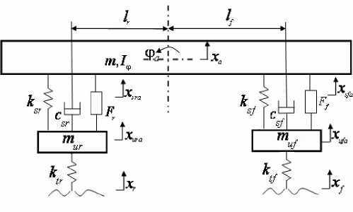
Figure 1. Active suspension of 4-DOF automobile model

In this paper we chose the parallel active suspension as research object and its model is shown in Fig.1 as in [7]. We select equilibrium positions of the suspended mass and the unsprung mass as their each origin of coordinates.

According to Newton's second law we can draw the following dynamics equations of the model uf ufa sf sfa ufa sf V sfa ufa / f tf x ufa f /

muAa - ksr (xsra - xura )

sr sra ura         r tr ura r

'                                                                       (1)

a sf sfa ufa          sf sfa ufa           f ф т a r L sr v sra ura / sr v sra ura / r f L sf x sfa ufa / sf x sfa ufa / f -I

rigidity coefficients of the front and rear suspensions. c_sf and c_sr respect the damping coefficients of the front and rear suspensions. I ^ is the pitching rotational inertia. F_f and F_r are the active control force of the front and rear suspensions. x_ufa and x_ura are the displacements of the front and rear wheel unsprung masses. x_sfa and x_sra are the displacements of the front and rear wheel sprung masses. x_a is the centroidal displacement of the car body. ф_a is the centroidal pitching angle of the car body.

Since the pitch angle is tiny, ф_a approximately equals

as the state variable and Y = ( x ,   ф ,   & ,   ф ,

a          a, a, a, a,

to tgф_a . We can also obtain an equation from the geometric relations of the model as follow

x , - x , , x - x , x, - x , , x - x ) T as the sfa ufa sra ura f ufa         r ura

x sfa

x

a

^™J

output variable. Then (1) can be transformed into the following state-variable equations as in

a aa a     a a aa a     a

Where the coefficient matrixes are

In (1) m is the mass of the suspension. lf and lr are the distances from the front and rear axles to the center of mass of the car. muf and mur are the unsprung masses of the front and rear wheels. ktf and ktr are the springs’

	" 0	0	0	0	1	0	0	0      "
	0	0	0	0	0	1	0	0
	0	0	0	0	0	0	1	0
	0	0	0	0	0	0	0	1
	Kr + k sf tf	0 k + k sr       tr	k sf	l f k sf	c sf	0 c sr	c sf	ic f sf
A = a	m uf 0		muf k r	muf lk r sr	muf 0		m uf c sr	m ic rr
		m ur	m ur	m ur		m ur	m ur	m ur
	k sf	k sr	k, + k sf      sr	- l k + l k ff rr	c sf	c sr	cr + c sf      sr	-Lc, + 1 c f sf r sr
	m lk f sf	m lk r sr	m Lk, - lk f sf     r sr	m 1 2 k, + 1 2 k f sf     r sr	m lc f sf	m lc r sr	m l c - l c f sf     r sr	m l f 2 c f + lr 2 c r
	I L       ф	I ф	I ф	I ф	I ф	I ф	I ф	I ф      J

■ 0	0         1             0           0      0        0             0      "
0	0        0            1          0      0        0            0
k-L m c = - 1Al a I ф - 1	k sr        k sf + k sr    - lfk f + lrksr      c sf       C sr        c sf + c sr    - lf c sf + lc r mm   m   m  m   m   m Ik l,k, - lk    1 2 kf + 1 2 k      l,c, lc l,c, - lc 1 2 c, + 1 2 c r sr f sf r sr f sf r sr           f sf         r c sr f sf r sr f sf r sr II  I  III  I ф             ф                   ф                 ф        ф            ф                  ф 0         1               lf           0       0         0             0
0	- 1         1              - lr          0       0         0             0
- 1	0        0            0         0      0        0           0
_ 0	- 1        0            0          0      0        0            0      _

								" 0	0 "
	0	0
								0	0
	0	0
	0	0
	0	0						m	m
	1 ^^^^^^™ ^^^^^^^^^^^^^^^^^^^^™	0				D	=	к	l r ^^^^^ ^^^^^^^^^^я
	m			,		a		I	I
B =	uf							ф	ф
a	0	1 ^^^^^^s ^^^^^^^^^в	-					0	0
		m	ur					0	0
	1	1
	—	1                                   1						0	0
	m	m
	l f	l r						[ 0	0 _
	I	I
	ф	ф
	■ 0	0 "			"0	0"
	0	0			0	0
	0	0			0	0
	0	0
					0	0
	ktf		, F =
E =	-^-	0	a		0	0
a	muf				0	0
		к
	0	tr			1	0
		m
		ur
	0	0			[°	1]
	. 0	0 .

And U = ( F f , F r ) T is the input vector of the front and rear controller force. The road roughness is approximately treated as white noise, w =( x & f , x & r ) ^T .

B. Passive Suspension of 4-DOF Automobile Model

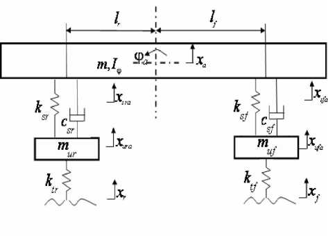
Figure 2. Passive suspension of 4-DOF automobile model

As previous, we can obtain the dynamic equations of the passive suspension model in Fig. 2 as follows m ,8k, - k , (X , - X, ) uf ufp sf sfp ufp sf v sfp ufp J     tf\ up     f / ur urp sr srp urp sr srp urp         tr urp r

p Sf \ sfp ujp/ sf \ sfp ufp ’

IД + lr [ksr (xs.p - xu.p ) + csr (^rp - ^urp )]

f sf sfp ufp          sf sfp ufp

According to the geometrical relationship, when the pitch angle is tiny, ф _p « tg ф _p , we can also obtain a similar equation as in the active suspension of 4-DOF automobile model.

transformed into the following state-variable equations as in

X p = A_pX_p + B_pw ( t ) Y_p = C p X p + D p w ( t )

X — X , X, — X , , X — X ) T . Then (3) can be srp urp f ufp r urp

Where w = (Xf, Xr)T and the coefficient matrixes are as follows

A p = C p = B = p

0        0         0          0        1      0       0          0     1 0    0     0     0    01    0     0 0    0     0     0    00    1     0 0    0     0     0    00    0     1 — k f + kf     о        k f        lk f       c f     о      cf        ^c f m     m   mm    m   m uf                                       uf                      uf                    uf                             uf                      uf k + k     k         Ik      c c     c         1c A         __ sr     r            r              __ r sr            A      __ sr            sr              __ r r m  m   m     mm   m ur                ur                     ur                              ur             ur                     ur k,       к       k, + k   —1k + 1k    c, c     c, + c   —Lc, + 1c sf                    sr                  sf      sr           f f     r r           sf             sr              sf      sr          f sf     r sr m   m    m   m   mm   m   m IX     Ik    1k — 1k  12 Ke + 1 2 k    lc lc   lc — lc  1 2 c, + 1 2 c f sf              r sr            f sf     r sr      f sf     r sr         f sf       r sr       f sf     r sr      f sf     r sr I     I     I      I     II    I      I ф            ф              ф                ф              ф       ф           ф               Ф      J " 0      0         1             0           0      0        0             0 00   0    1    00   0    0 ksf       k sr        kf + ksr    — 1fksf + 1r k sr      c sf       csT        c sf + c sr     - 1fcsl + 1, mm  m   m   mm  m   m —    hk f    1 r k sr    1 f k sf — 1 r k sr    1 f2 k f + 1 r2 k sr   — 1fc f    1rcsr   1fc f — 1rcsr   1f2 c f + 1„ II   I     I    II   I     I ф        ф             ф                   ф                 ф        ф            ф                  ф — 10     1         1f      0    0     0        0 0       - 1        1             - 1r          0      0        0             0 - 1     0        0            0         0      0        0           0 _   0      — 1        0            0          0      0        0            0 Г 00 1     Г0 01 0    0            0  0 0    0            0  0 0    0            0  0 kf       , DB = -f  0       p 0 0 m "ft            0  0 0 k^     10 m„          1   0 00       Lo 1J _ 0     0 _

c c -J r.

• III.    D ESIGN O F T HE VSMFC F OR T HE A CTIVE S USPENSIONS

• A.    Reference Model

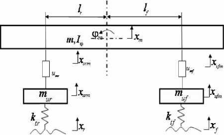
Figure 3. Suspension of the reference model

To build the VSMFC system, we select the independent active suspension based on optimal control method as the reference model which is obtained by removing the passive spring and damping units in Fig. 3. According to the 4-DOF dynamical equation of the parallel active suspension, we can get the reference model of independent active suspension with the same order. The dynamics equations of the model are as follows uf ufm fm tf ufm f m fm rm

Ф rm r rm f fm

And the state-variable equations of the reference model are as in m mm mm m m mm mm m

Optimal control theory, described in the text, is how to ensure the performance index of the suspension system to be optimal under the conditions defined in the first equation of (6). Owing that the suspension system need to ensure the ride comfort, running stability and security in the parameter requirement aspects, we adopt body displacement, body acceleration, suspension and tire deformation (or dynamic tire load) as the objective functions. Here we use the output feedback of the infinite time regulator and select the performance index function of the active suspension as follow

= "\YTQY + UTrU 1 dt                (7)0m m mm

= "ГXTQ'X + UTRU + 2X TNU 1 dt 0m   m mm    m m

In (7), qixm , L , q8(xr -xurm)2     are the correspondences to each output performance index. r1u2fm andr2u2rm correspond to the two input controller forces. q1, l , q8, r1, r2 are the weighted coefficient which are determined by different requirement level of the performance index.   Q = diag(q1,L , q8) ,

r = diag(ri,r2), Q' = CmQCm R = DmTQDm + r , N = C TQD . mm

Using the variation method we obtain the following optimal feedback form, U m =-KX m , K=R^- 1 ( B m P + N T ) , in which P is the positive definite solution of the Riccati matrix equation.

• B.    Selection of the Expected Close-Loop Pole Set for Pole Assignment

The first step for a pole assignment problem is to select the expected close-loop pole set reasonably. As the performance index, the expected close-loop pole set has its two sides. Setting the expected close-loop pole set as the performance index makes it concise and strict to establish the corresponding theory and arithmetic in view of control theory. However, in view of control engineering that should be unacceptable for intuitionism deficiency. For these reasons, corresponding relations between intuitionism and the expected close-loop pole set must be built to make it acceptable for both control engineering and control theory.

• 1)    Dynamic Property and Index of the System

In order to assess the performance of the linear system in time domain, we should analyze the time domain response of the system with some typical signal inputs. If the dynamic performance of the system with a step signal input can meet the requirements, the response of the system would be satisfactory with the other forms of signal inputs.

The transfer function of a generic second-order system can be written as

When

to

n

(systemic undamped natural

frequency), Z =-------(systemic damping ratio), and 2ton • a equation can be rewritten as

ф( 5 ) =

to ²

n

5 ² + 2Zto . 5 + to 2 .

It's the standard form of the transfer function of a generic second-order system, the characteristic equation of which is

And the two poles are 5 1 2 = —Zto _n ± j to _n ^ 1 — Z 2 , that indicates the poles vary when the damping ratio changed. Usually, the system is expected to running in underdamping condition ( 0 < Z < 1 ) when the system could provide proper concussion and shorter transient process.

For convenient analysis and comparison, suppose the system is standstill before unit step inputting, and that output as well as its derivatives are all zeros. The response of the second-order system in underdamping condition is demonstrated in Fig. 4.

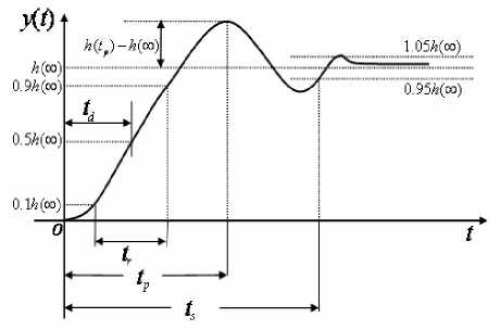
Figure 4. Response index for unit step input

The dynamic performance indexes are as follows:

• a)    Delay time t_d , time cost by the response curve achieves half of its final value for the first time .

• b)    Rise time t_r , time cost by the response curve rises from 10% of the final value to 90% of that. For the oscillation system, the rise time can also be defined as the time taken by the curve to rises from zero to its final value for the first time. Rise time reflects the response speed; shorter rise time means more quickly response .

  t = П—Р = r

  
  

  <У

  c

  
  

L_

• c)    Peek time t_p , time cost by the response curve achieves its first peek value .

  t p

  
  

  П

  4 71— 4 ’

  
  

• d)    Regulating time t_s , the time taken by the curve to achieve and keep in the bounds of ±5% (or ±2% ) of the final value. Regulating time reflects the inertance of the system, and also the speed of response .

• e)    Overshoot < 7 % , ratio of the difference between the maximum offset of the response and the final value to the final value, that is

And if h ( t_p ) <  h (да) , there is no overshoot in the response.

The five indexes above can mainly reflect the dynamic characteristic of the system. In practical application the rise time, regulating time and overshoot are most commonly employed.

• 2)    Fundamental of the Selection of Expected Closeloop Pole Set

The property of a control system is mainly depending on the distribution of the poles on the radical plane. For this reason, in the design of a control system, the distribution of the poles is often determined according to the requirement of the properties. The so-called pole assignment is to assign the poles the wanted position by selecting a suitable feedback matrix K , in order to obtain an expected dynamic performance. The selection of the expected poles should meet the cardinal rules as below:

• a)    For an n dimension control system, the number of the poles could be and must be n.

• b)    In high-order system, only a fraction of the poles are decisive to the performance, which are called dominant poles and selected to replace the entire of the poles. The dynamical transition component generated by the non- dominant poles will be attenuated with celerity .

• c)    Both real and complex form of the pole is acceptable, but when it is complex, only the conjugate complex number is logical which is physically realizable .

• d)    In the selection of the position of the poles, both the effect to the system and the relationship with the distribution of the zero points should be taken into consideration .

• e)    The expected poles should be selected with an eye to the requirement of anti-interference capability and low sensitivity .

• C.    Select of the Switching Function

If the controlled system tracks the reference system accurately, their coefficient matrixes meet the full matching conditions of the model tracking system defined in [1]. That is and active controller force vector U can be obtained at this time.

From (2), (4) and (10), we can obtain the following differential equation of the active suspension system’s tracking error vector e = X m — X_a as

e X — X ma

= AX + BU — AX — BU (11)

mm mm aa a

= Ae + (A — A )X + BU — BU m     m a a mm a

We suppose that the switching function of the error system is s = Ce and use the block matrix to indicate it.

A m

f A^{11 m}

I A ^{21 m}

A ¹²) ^m

A²² J

m

^, e ⁽ e l e 2 ) ^,

In the above equations, A_m ¹¹ is a six-by-six matrix. e ₁ ,

C ₁ and T ₁ are six-by-one matrixes. We make a linear transformation, % = Te , and let T ₁ B equal zero. Then (11) can be transformed into the following form as

%= TAT—1 e + T(A — A )X + TB U — TB U (12) m          m a a mm a

And we can obtain the simplified form of the sliding mode equation of the error system when the matching condition of the model tracking, and the sliding model condition, s = C % + C ₂ % = 0 , are both satisfied .

The simplified form is as follow

% = > % + > % = ( > — > C <%) %

In the error system, (A, B) is controllable pair and the transformed coefficient matrix (A11, A12) is also a mm controllable pair. So we can find a matrix K = C— C to make (Aу — A“ K ) having the required poles, Я, Л, Я6 .That is to say that the roots of the equation 11 Я — (A1 — A^2 K )| = 0 are all in the left-half plane and n—m        m m the poles can be configured. After determining the K, we can obtain the coefficient matrix C% which can be introduced in the following form: C = [ %, C2] = [ C2 K, C2] = C2[ K, 12].

We usually set C ₂ equal as I _m , then we can obtain the equation C = [ K , I_m ] . And the matrix C ^% can be transformed into C , the switching function matrix of the error system, through the matrix T .

• D.    Hierarchical Algorithm of Control Variables Startup in Sequence

The controlled system is a dual-input system. In order to reduce the number of online solving equations and improve the response speed of the system we adopt a hierarchical algorithm of control variable startup in sequence as in [8].

Making s ₁ = 0 under the sliding mode first and then we use the exponential reaching law to calculate the controller force F_f of the front suspension .The equation is shown as follow:

Where 8 ₁ and k are adjustable parameters. With the

8 ₁ decreasing, the inertia is decreased to reduce the chattering and the dynamic quality of the approaching mode ( S ₁ ^ 0 ) may be increased. So we could increase k ₁ to reach the switching surface fast and the equations of the system are shown as follow as in [9]:

f <&= Ae + ( A — A XX + B U — B F, m \ m a J a mm    a 1 f (14)

_ ^s 1 = C 1 ^e

In (14), C1 is the first line of C and Bal is the first column of Ba are vectors. Equation (13) substituting (14) will be changed into the following form:

ds- = —81 sign(s1) - s1dt

The active controller force equation suspension is as follow:

^B a 1 F , )

of the front

^F, = ( CB a 1 )

- 1

The following controller force:

CA e + C(A — A XX

1 m         1 m a a

is the equation of the equivalent

^F,e, = ( ^C 1 ^B a 1 ''

C1 Ame + C1 ( Am — Aa ) Xa +C1 B.U.

With starting the control force F_r the dynamic equations of the sliding mode are transformed into the following form:

m         m a a m m a1 f a2 r ds2

We use Ffeq instead of Ff and suppose d 2 to be zero in the sliding mode s2 = 0 . Then the conclusion can be described as follow:

F = ( CB₉) req          2 a 2

CA e + C2(A — A )X

2 m        2 m a a

+C B U - C B F

2 m m 2 a 1 feq

So we can conclude the following equation:

F r = ( C 2 B a 2 )

C A e+C,(A - A )У

2 m        2 m a a

+CB U -CB F

2 m m 2 a 1 feq

+E2 sign (s 2)+k2 s 2

And then we can achieve VSMFC for dual-input active suspension by using (19) and (20).

• IV.   S IMULATION A ND A NALYZE O F T HE R ESULTS

The parameters of a mini-car model are listed in Table I. After being verified, the dynamic model matched the conditions of the model following system perfectly.

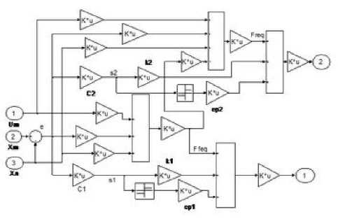
Figure 6. The Subsystem of variable structure model following control systems

TABLE I.

P ARAMETERS O F A M INI -C AR M ODEL

lf / mm	l / mm r	m / kg	muf / kg
1222	1126	389.5	30.4
k / kN sf	k sr / kN	k / kN tf	k tr / kN
30	32.5	425	425
mur / kg	I ф / kg • m 2	c f / N • s / m	csr / N • s / m
31.7	2251.34	3300	3300

• A. Comparison and Analysis of the Simulation Results

The simulation results of body acceleration, body pitch acceleration, suspension working space (SWS) and dynamic displacement of tire are shown from the Fig. 7 to Fig. 12.The results indicate that the performance indicators of the front and rear suspension have improved besides that the dynamic deformation of the rear wheel has increased. The comparison of the root-mean-square value of output between active suspension and passive suspension is shown in table I, where the simulation results of pre-10s are collected.

Take B-class road as the input. The road roughness coefficient G q ( n 0 ) is 64 x 10 ⁶ m 3 and the vehicle speed u is 20 m / s . Reference spatial frequency n ₀ is 0.1 m ¹ and the power spectral density of velocity is a white noise as follow:

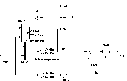
Build a simulation model of the system in Matlab/Simulink as shown in Fig. 5 and Fig. 6.

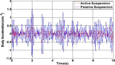
Figure 7. The result of body acceleration.

VSMFC

Passive suspension

Figure 5. The structure of variable structure model following control systems

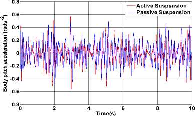
Figure 8. The result of body pitch acceleration.

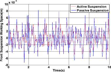
Figure 9. The result of front SWS.

Root-mean-square	Passive suspensions	Active suspensions	Depression rate (%)
Body acceleration (m/s 2 )	4.20e-3	1.50e-3	64.29%
Body pitch acceleration (rad/s 2 )	1.60e-3	1.40 e-3	12.50%
Front SWS (m)	2.67e-5	2.05e-5	23.22%
Rear SWS (m)	3.27e-5	2.04e-5	37.61%
Front DDT (m)	6.54e-6	5.59e-6	14.53%
Rear DDT (m)	6.64e-6	7.50e-6	-12.95%

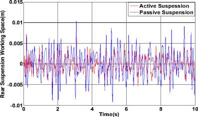
Figure 10. The result of rear SWS.

₃ x 10^-3

Е

Е

Active Suspension

Passive Suspension

till! MWIi^il^kMWIl

-2

-3 ь

-40

46 Time(s)

Figure 11. The result of front DDT

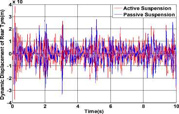
Figure 12. The result of rear DDT.

TABLE II.

M EAN SQUARE ROOTS OF SIMULATION RESULTS

Root-mean-square

Passive suspensions

Active suspensions

Depression rate (%)

We can see that the remaining indicators fell down by 64.29% 、 12.50% 、 23.22% 、 37.61% 、 14.53% besides the dynamic deformation of the rear wheel has increased. But we can also see that the dynamic load of rear wheels has increased by 12.95%, which has affected the safety. We should take a balanced consideration of all factors when design the reference model, and the control system parameters should be properly adjusted to obtain better overall performance suspension.

B. Analysis of the Following Performance.

The designed controller is a model tracking controller which is implemented by variable structure control, so it is necessary to analyze its following performance. Here we select the state values of the reference and controlled system to show the following performances.

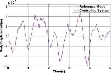
Figure 13. Displacement between reference model and controlled

system

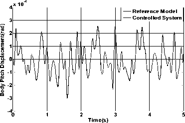
Figure 14. Pitch displacement between reference model and controlled system

Fig. 13 and Fig. 14 show the comparison results of the two systems represent the body displacement and body pitch displacement. From the figures we can see that the controlled system imposed the active control force can accurately track the state values in a very short time. Then we can draw the conclusion that the following performance of the controller is good and the system responses rapidly.

C. Analysis of the Robustness.

For the control system design, robustness is one performance must be met. The uncertain factors of the suspension system are mainly from two aspects. The first is the uncertain driving conditions such as the redistribution of the car load caused by turning or braking. The second is the changes of the car parameters such as the changes of the car load, the influences on tire stiffness from the inflation pressure, temperature and the degree of aging. Although the uncertainties from two aspects, they are all the reasons causing the changes of the model parameters from the dynamic perspective. So in this paper, we use the changes of the body mass and the stiffness of the tire to verify the robustness of the active control system. We change the parameters of the controlled system by increasing or decreasing the body mass and the tire stiffness by 20% to observe the changes of the output where we only select the body displacement and pitch angle to explain the output results. The simulation results are shown in Fig. 15 and Fig. 16.

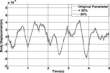
Figure 15. Results of body displacement under different parameters

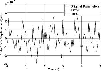
Figure 16. Results of body pitch displacement under different parameters

From the results we can conclude that VSMFC has a high degree of robustness and the change and disturbance of the model parameters have a strong adaptability.

• V.   C ONCLUDING R EMARKS

In this paper, we select the 4-DOF vehicle vibration model as the basis for research and we take the independent active suspension as reference model. Then we built a variable structure model following controller of the parallel active suspension system and establish the simulation model of the controller in the Matlab/Simulink.

The simulation results show that the model following variable structure controller can significantly improve the body acceleration and ride comfort. At the same time it can reduce the SWS and the dynamic displacement of tire to improve the handling stability and driving safety of the car. The designed active suspension control system is not only responsive but also has a high degree of robustness and a strong adaptability.

The control algorithm discussed in the paper not only provides an important theoretical basis for the design of the active suspension but also has a certain reference value for the design of the active control system such as the chassis.

A CKNOWLEDGMENT

We would like to thank the editor and the reviewers for their consideration. We also acknowledge the support by the Natural Science Foundation of Shandong Province, China (2R200PFL016).