Вариации интенсивности мюонов и температура атмосферы

In recent years, the number of muon telescopes for cosmic ray (CR) observation has gone on increasing [Osipenko et al., 2015] . This is due to a variety of their advantages as compared to neutron monitors [Yanchu-kovskiy, 2010] . There is, however, a deterrent as well — the presence of the temperature effect of muons in the atmosphere. Its correct consideration in continuous observations made with muon telescopes requires us to know the distribution of temperature coefficient density for atmospheric muons and the atmospheric temperature profile at a given time. The distribution has been found from calculations [Kuzmin, 1964; Dorman, Yanke, 1971; Dmitrieva et al., 2009; Kuzmenko, Yanchukovsky, 2017] and evaluated using continuous long-term observations [Yanchukovsky, Kuzmenko, 2018] . The results allow us to consider the temperature effect in data from muon telescopes as shown in [Osipenko et al., 2015] . The main difficulty in the correct consideration of the temperature effect arises from the quality of aerological data. The aerological sounding is made twice a day and not at the telescope site — a sounder may be up to hundreds of kilometers or more away. Sounders often do not make full measurements because they do not reach desired heights, thus the measurements have gaps. Data is therefore often obtained from interpolation and extrapolation. Measurements of the muon intensity with the telescopes are made at a high statistical accuracy and resolution of 1 hr, in most cases 1 min (with some telescopes, 1 s). Consequently, a question arises as to how to consider the temperature effect in observations of muon telescopes without aerological data.

TIME VARIATIONS OF COSMIC RAY MUON INTENSITY

Variations in the intensity of different CR compo- nents, detected by the channel k at h0 in the atmosphere at the site C with geomagnetic cutoff rigidity Rc, are composed of intensity variations in the primary CR flux

D ( Rt >

of magnetospheric and atmospheric origin

[Dorman, 1975]

^k" ( h ₀, t ) =

Ik c

= J A D ( R , t)W_k ( R , h o ) dR -^ R _c( t)W_k ( R _c, h 0 ) + (1)

R c ^D

+ <  exp

jpk(h)dh ho

-1U

h j wk (h, h)AT(h, t)dh.

Here, W k ( R , h 0 ) is the coupling coefficient of k according to the definition [Dorman, 1975] ; β k ( h ) is the barometric coefficient of k ; w ( h 0 , h ) is the temperature coefficient density function, Δ T ( h , t ) is the atmospheric temperature variations with time and height. The atmospheric component of the intensity variations includes barometric and temperature effects (the third and fourth terms of the expression).

In case of simultaneous observations of several CR components in different energy ranges, the observed variations are disaggregated using a spectrographic method [Dvornikov et al., 1979] , adapted for CR multichannel detection at one site [Yanchukovsky et al., 2011] . We can also employ statistical methods, representing Expression (1) as a multivariate regression equation [Yanchukovsky, Kuzmenko, 2018] . Thus, the multichannel recording of different CR components at one site allows us to also identify the temperature component of muon intensity variations by solving (1). This was first shown in [Yanchukovsky et al., 2011] . At a given temperature variation of the muon intensity

A I k

I k

(T, t), we can solve the inverse problem — deter- mine temperature variations at various isobars in the atmosphere from the system of equations

h

—T ( T, t ) = J w_k ( h )A T ( h , t ) ^h .

Ik           0

In this way, variations in 11 isobars over a long period have been found and compared with aerological data [Yanchukovsky et al., 2015] . The integral in Expression (2) was replaced by the sum, and w k ( h ) was tabulated as temperature coefficients. The temperature coefficients of intensity in use were derived from experimental data for particular isobars. Note that a further increase in the number of isobars, which requires determining temperature variations, is limited by the number of muon recording channels in this case.

DISTRIBUTION

OF TEMPERATURE COEFFICIENT DENSITY FOR ATMOSPHERIC MUONS

To take into account the temperature effect in data from muon telescopes and when solving the inverse problem, it is desirable to use the experimentally obtained distribution of temperature coefficient density since it corresponds to a particular device and is free of various approximations specific to theoretical methods. Yanchu-kovsky, Kuzmenko [2018] have found the distributions of muon intensity temperature coefficient density recorded at different zenith angles, using different multivariate analysis methods. Table 1 lists distributions of temperature coefficient density for muons recorded without a lead shield (O.I.) and with a lead screen at zenith angles of 0°, 30°, 40°, 50°, 60°, 67°, and 71°, found as an average obtained by the PLS -2 method (KERNEL algorithm) and the correlation and regression analysis.

Using data from Table 1, we have approximated the w ( h ) distributions with the polynomial. The approximation was carried out using the least squares method (LSM). Figure 1 shows the obtained distributions of w ( h ) for channels of vertical recording of muons (0° to the zenith) without a lead shield ( a ) and with a lead shield providing a muon cutoff energy of 0.56 GeV ( b ), and under zenith angles of 30° ( c ) and 40° ( d ).

In a similar way, we approximated temperature coefficient density distributions for muons recorded at zenith angles of 50°, 60°, 67°, and 71°. The results are presented in Figure 2.

For all directions of muon detection (under different zenith angles) the density distribution of temperature coefficients shown in Figures 1, 2 is best described by the function that is the sixth degree polynomial w (h) = a0 + axh + a^h2 + a3h3 + +a4h4 + a5h5 + a6h6.

The approximation function parameters, polynomial coefficients a 0 , a 1 , ..., a 6 found by LSM are presented in Table 2.

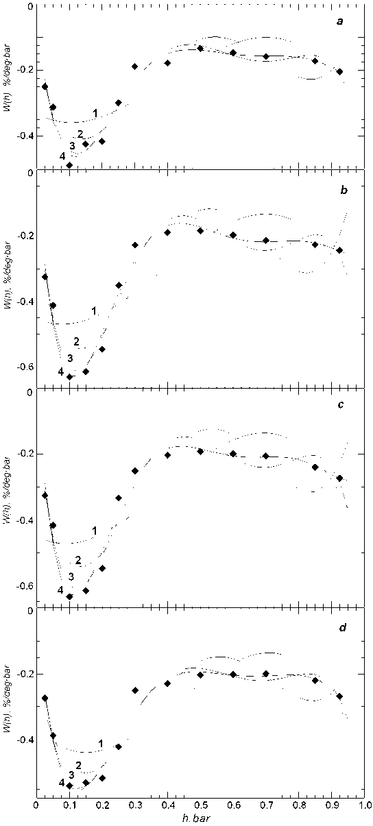
Figure 1 . Approximation of temperature coefficient density distributions for muons detected vertically (0° to zenith) without a lead shield ( a ) and with a lead shield, which provides a muon cutoff energy of 0.56 GeV ( b ), and at zenith angles of 30° ( c ) and 40° ( d ). Curve 1 is the polynomial of degree 3; curve 2, the polynomial of degree 4; curve 3, the polynomial of degree 5; curve 4, the polynomial of degree 6

VERTICAL DISTRIBUTION OF ATMOSPHERIC TEMPERATURE

We have used aerological data obtained from January 1, 2004 to November 7, 2018 (10849 launches) []. Table 3 lists average temperatures at different isobaric levels of the atmosphere obtained for the entire period for different seasons, and also shows the number of measurements in use.

Table 1

Muon intensity temperature coefficient density in the atmosphere w ( h )

h , bar	O.I.	0°	30°	40°	50°	60°	67°	71°
0.05	–0.313	–0.412	–0.415	–0.387	–0.445	–0.469	–0.703	–0.479
0.1	–0.489	–0.629	–0.632	–0.540	–0.762	–0.639	–0.879	–0.598
0.15	–0.425	–0.613	–0.613	–0.531	–0.760	–0.630	–0.726	–0.494
0.2	–0.416	–0.545	–0.546	–0.518	–0.728	–0.579	–0.671	–0.457
0.25	–0.300	–0.351	–0.332	–0.422	–0.426	–0.400	–0.619	–0.421
0.3	–0.189	–0.228	–0.251	–0.250	–0.295	–0.304	–0.319	–0.217
0.4	–0.178	–0.191	–0.203	–0.230	–0.231	–0.245	–0.180	–0.122
0.5	–0.134	–0.186	–0.191	–0.204	–0.216	–0.234	–0.108	–0.073
0.7	–0.159	–0.215	–0.205	–0.199	–0.243	–0.175	–0.102	–0.070
0.85	–0.172	–0.227	–0.239	–0.220	–0.294	–0.231	–0.139	–0.095
0.925	–0.205	–0.245	–0.272	–0.268	–0.301	–0.280	–0.184	–0.153

Here, w ( h ) is in %/(deg. bar).

Table 2

Parameters of approximation function of temperature coefficient density distributions for muons recorded at different zenith angles θ

θ	а 0	а 1	а 2	а 3	а 4	а 5	а 6
O.I.	–0.0363247	–9.256169	67.184662	–196.71242	283.05153	–199.37579	54.90318
0°	–0.0001308	–13.86269	102.53497	–304.70426	442.38944	–313.35752	86.74166
30°	0.00461710	–14.17922	106.82805	–326.53205	490.75341	–361.18261	104.0522
40°	–0.0425815	–10.35925	70.729137	–195.81495	265.18775	–173.95738	43.86181
50°	0.19893443	–20.59934	147.67809	–439.1849	648.04104	–471.58344	135.2362
60°	0.06428264	–16.01382	121.3395	–384.67404	607.13936	–470.57117	142.5278
67°	–0.0998818	–16.44955	120.34995	–350.7992	508.00637	–364.5099	103.3406
71°	–0.0627640	–11.25749	81.84462	–236.3424	337.35257	–237.10135	65.35399

Table 3

Average atmospheric temperatures (in °C) in isobars for different seasons

h , bar	T , °С					Number of measurements n
	Winter	Spring	Summer	Fall	Year	Winter	Spring	Summer	Fall	Year
0.01	–46.25	–43.08	–38.32	–47.50	–43.79	228	886	1266	750	3130
0.02	–53.54	–51.66	–45.25	–54.70	–51.29	838	1665	1921	1497	5921
0.03	–58.47	–54.67	–48.61	–57.68	–54.86	1289	1851	2057	1805	7002
0.05	–61.95	–56.30	–50.81	–58.80	–56.96	1830	2113	2246	2113	8302
0.07	–62.45	–56.43	–51.42	–58.11	–57.10	2086	2248	2341	2255	8930
0.1	–61.73	–55.65	–50.90	–57.13	–56.35	2237	2394	2425	2346	9402
0.15	–60.86	–54.47	–49.05	–56.15	–55.13	2318	2473	2500	2428	9719
0.2	–62.15	–56.30	–50.41	–57.32	–56.54	2387	2529	2556	2482	9954
0.25	–61.29	–55.99	–49.68	–55.89	–55.71	2426	2571	2585	2526	10108
0.3	–56.47	–50.85	–42.53	–50.00	–49.96	2470	2600	2606	2569	10245
0.4	–44.27	–37.59	–27.21	–36.17	–36.31	2506	2626	2631	2595	10358
0.5	–33.59	–26.33	–15.41	–24.86	–25.05	2526	2647	2649	2614	10436
0.7	–18.65	–10.71	0.54	–9.58	–9.60	2541	2672	2699	2636	10548
0.85	–13.01	–2.58	10.31	–2.39	–1.92	2549	2684	2714	2645	10592
0.925	–12.91	1.33	15.75	0.81	1.24	2549	2684	2715	2646	10594

Here: winter — December–February; spring — March–May; summer — June–August; fall — September–November.

The vertical atmospheric temperature distributions obtained from these data over Novosibirsk (annual average and for summer and winter seasons) are shown in Figure 3.

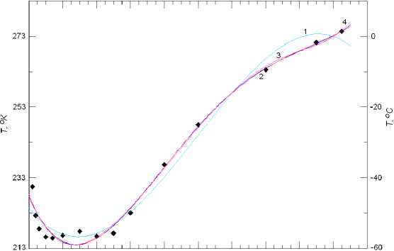
The atmospheric temperatures for spring and autumn seasons are close to annual average ones (curve 1). The approximation of the average atmospheric temperature distribution is illustrated in Figure 4.

Curves 2–4, which represent the polynomials of degree 4–6, virtually coincide. The distribution of average seasonal temperature variations Δ T ( h ) as a function of atmospheric depth h is shown in Figure 5.

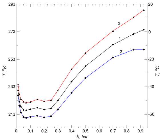
Figure 3 . Vertical distribution of atmospheric temperature: Annual average — curve 1; for summer — curve 2; for winter — curve 3

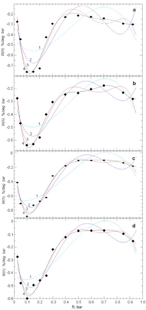
Figure 2 . Approximation of temperature coefficient density distributions for muons recorded at zenith angles of 50° ( a ), 60° ( b ), 67° ( c ), and 71° ( d ). Curve 1 is the polynomial of degree 3; curve 2, the polynomial of degree 4; curve 3, the polynomial of degree 5; curve 4, the polynomial of degree 6

0       0.1      0.2      0.3      0.4      0.5      0.6      0.7      0.8      0.9     1.0

Figure 4 . Approximation of annual average atmospheric temperature distribution: polynomial of degree 3 (curve 1), polynomial of degree 4 (curve 2), polynomial of degree 5 (curve 3), and polynomial of degree 6 (curve 4)

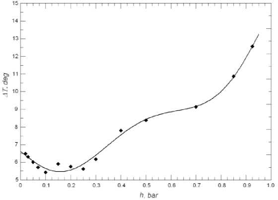
Figure 5 . Vertical distribution of atmospheric temperature variations: dots indicate experimental data; the solid line is the approximation of the dependence by the sixth degree polynomial

Table 4

Parameters of approximation function for distribution of observed temperature variations (averages) from the depth of the atmosphere

b0 b1 b2 b3 b4 b5 b6 6.638635 –14.810158 65.654888 –28.445272 –129.468102 158.636595 –42.541395 c 3 k = 1 a 0 kh 4 + 1 alkh 5 + 1 a 2 kh 6 + 1 a3 kh 7 +

The experimental dependence Δ T ( h ) is approximated using LSM. The sixth degree polynomial best satisfies all the experimental values

A T ( h ) = b 0 + b 1 h + b 2 h ² + b 3 h ³ + b 4 h ⁴ + b ₅ h ⁵ + b 6 h 6 .   (4)

Approximation function parameters, polynomial coefficients b 0 , b 1 , ..., b 6 are presented in Table 4.

DETERMINING TIME

VARIATIONS IN THE

ATMOSPHERIC TEMPERATURE FROM DATA ON MUON INTENSITY VARIATIONS

Using (2), set w k ( h ) and Δ T ( h , t ) functionally with polynomials (3) and (4), whose product also yields a polynomial. Then, integral (2) is transformed into the sum of integrals in which the integrand represents a power function. As a result, the system of k integral equations can easily be transformed into a system of k linear equations of the form

^A I^{k ( T} , t ) = c 0 k b 0 ⁽ t ) ⁺ c l k^b1 ⁽ t ) ⁺ c 2 k b 2 ⁽ t ) ⁺

Ik

⁺ c 3 k b 3 ⁽ t ) ⁺ c 4 k b 4 ⁽ t ) ⁺ c 5 k^b 5 ⁽ t ) ⁺ c 6 k b 6 ⁽ t ),

where c 0 k , c 1 k , ..., c 6 k are the constant coefficients specific to k , which can be found as

c 0 k    a 0 k h + 2 a 1 k h + 2 a 2 k h		1 4 +— a^h 4   3 k			+
1       51       6 + - a 4 k h + - a 5 k h 56	17 + y a 6 k h ,
1        2 1        3 1 c 1 k   2 a 0 k h + 2 a 1 k h + Д a 2 k		h 4 +	1 5	a 3 k	h 5	+
1       61       7 + - a 4 k h + -a 5 k h 67	+— a^h 8 , 8   6 k   ,
1        3 1        4 1 c 2 k = ^ a 0 k h + д a 1 k h + ^ a 2 k		h 5 +	1 6	a 3 k	h 6	+
+ - a 4 k h 7 + 7 a 5 kh8 78	1 9 + g a 6 k h ’

1        8    1        9     1

+ 7 a4kh  '   a5kh + 77 a6kh’

8        910

c 4 k = 7 a 0 k ^{h +} 7 a l k ^{h +} 7 a 2 k ^{h +} 7 a 3 k ^{h +} 5678

1        9     1         10     1

+ g a4kh  + |() a5kh  +YTa6kh ’ c 5 k = 1 a 0 kh 6 + 1 al kh 7 + 1 a 2 kh 8 + 1 a 3 kh 9 + 6789

1         10     1         11     1

+ — a 4 kh + “a 5 kh + ^a 6 kh, c6k = 1 a0kh7 + 1 a1 kh8 + 1 a2kh9 +   a3kh‘° +

7        8        9        10

1         11     1         12     1

+ Y7 a4kh +^ a5kh  + ^a6kh■

Here a 0 k ; a 1 k , ..., a 6 k are the coefficients listed in Table 2, h =0.95 bar. The constants c _{0 k} , c _{1 k} , ..., c _{6 k} specific to each of the k telescope channels and found according to (6) are presented in Table 5.

The vertical distribution of atmospheric temperature variations for a moment t is described by a polynomial with the coefficients b 0 ( t ), b 1 ( t ), ... b 6 ( t ), which are determined by solving system of k linear algebraic equations (SLAE) (5). For “good” SLAE, i.e. described by a squared well-conditioned matrix A , there is an only solution, which can easily be found numerically, for example by the Gauss method. During processing of experimental data, the matrix A is, however, not squared (in case of an inconsistent, overdetermined system) or ill-conditioned (errors in matrix coefficients and left sides — experimental data as well as rounding errors).

As a result, if there is noise, SLAE with a rectangular matrix have no solution. It is therefore common practice to search for pseudosolution, not for exact solution (because it does not exist). In this case, the solution of SLAE is replaced by the problem of finding a global

Table 5

Parameters c _{0 k} , c _{1 k} , ... c _{6 k} , telescope channels

θ	c 0	c 1	c 2	c 3	c 4	c 5	c 6
O.I.	–0.21181	–0.08269	–0.04933	–0.03491	–0.02703	–0.021559	–0.017915
0°	–0.273062	–0.10648	–0.063587	–0.045123	–0.034777	–0.027648	–0.022751
30°	–0.276809	–0.10887	–0.065543	–0.04667	–0.03614	–0.028973	–0.023917
40°	–0.271589	–0.108562	–0.064627	–0.045702	–0.035035	–0.028119	–0.023239
50°	–0.327214	–0.129324	–0.077364	–0.055101	–0.042372	–0.033943	–0.028067
60°	–0.2918065	–0.112311	–0.065629	–0.045944	–0.0351678	–0.028196	–0.0233705
67°	–0.286174	–0.084089	–0.042739	–0.028655	–0.021608	–0.017559	–0.014566
71°	–0.19585	–0.058676	–0.030347	–0.020796	–0.015917	–0.012999	–0.0109328

(total for the entire system) minimum of the residual function f(x )=|Ax - b |. Since this minimized rate depends on the sum of squared components of the vector, the search for pseudosolution is an implementation of LSM [Kalitkin, 1978]. This yields a system of normal equations, which in the matrix form is or AB(t)=D(t). The coefficients of the matrix A reflecting characteristics of channels of muon intensity detection are found as follows:

a 00 a 01 a 02 a 03 a 04 a 05 a 06	b 0( t )		d 0 ( t )
a 10 a 11 a 12 a 13 a 14 a 15 a 16	b 1( t )		d 1( t )
a 20 a 21 a 22 a 23 a 24 a 25 a 26	b 2( t )		d ( t )
a 30 a 31 a 32 a 33 a 34 a 35 a 36	b 3( t )	=	d 3 ( t )	(7)
a 40 a 41 a 42 a 43 a 44 a 45 a 46	b 4( t )		d 4 ( t )
a 50 a 51 a 52 a 53 a 54 a 55 a 56	b 5( t )		d 5( t )
a 60 a 61 a 62 a 63 a 64 a 65 a 66	b 6( t )		d 6 ( t )

n n a00 = E k=1 c02k ,a 01 = a10 =E k=1 c0kc1k, n n a02 — a 20 = E k=1 c0kc2k, a03 = a30 = E k=1 c0kc3k, n n a04 — a40 = E k=1 c0kc4k, a05 = a50 = E k=1 c0kc5k, n n a06 = a60 = E c0k c6k, a11 = E Ck, nn a12 = a21 = E C1 kC2k , a13 = a31 = E C1 kC3k , k=1                              k=1

nn a14 = a41 = E C1 kC4k , a15 = a51 = E C1 kC5k , k=1                              k=1

nn a16 = a61 = E C1 kC6k , a22 = E C2k , k=1

nn a23 = a32 = E C2kC3k , a24 = a42 = E C2kC4k , k=1

nn a25 = a52 = E C2kC5k , a26 = a62 = E C2kC6k , k=1

nn a33 = E C3k , a34 = a43 = E C3kC4k , k=1

nn a35 = a53 = E C3kC5k , a36 = a63 = E C3kC6k , k=1

nn a44 = E C4k , a45 = a54 = E C4kC5k , k=1

nn a46 = a64 = E C4kC6k , a55 = E C5k , k=1

nn a56 = a65 = E C5kC6k, a66 = E C6k. k=1

Absolute terms D are d o( t) = ECо kJk (t),d 1( t) =EC1 kJk(t), k=1

d 2( t ) = EC 2 kJk ( t ), d 3( t ) = ]LC 3 kJk ( t ), k=1

nn d4(t) = E C4kJk (t), d5(t) = E C5kJk (t), k=1

n d 6( t)=EC 6 kJk(t).

k = 1

Here J (t) = —- (t) are the observed muon intensity Ik variations in k channels.

By solving (7), find the unknown parameters b 0 ( t ), b 1 ( t ), ..., b 6 ( t ).

RESULTS

We have used hourly continuous observations of muon intensity [] made with the matrix muon telescope [Yanchukovsky, 2006] in Novosibirsk in 2004-2011. The muon intensity data for each of the zenith angles was integrated over all azimuth directions. Thus, information was obtained about intensity variations for eight channels: muons recorded without a lead shield (O.I.) and with a lead shield at zenith angles of 0°, 30°, 40°, 50°, 60°, 67°, and 71°. To isolate the temperature component of the muon intensity variations, raw data was corrected for the barometric effect and the temperature effect, caused by surface (variable-density layer) temperature variations, and the variations attributed to primary CR flux variations were also taken into account [Yanchukovsky, Kuzmenko, 2018]. Since with increasing zenith angle the statistics decreases, measurements in the channels are unequal. To ensure the transition to the system of equilibrium equations, the data was smoothed using a moving average, where the step and order of smoothing were selected based on the distribution of statistical weights of channels. From the solution of (7), we determined unknown b0(t),b1(t), ..., b6(t). Then we found temperature variations in isobars

A T ( h , t ) = b ₀( t ) + b 1 ( t ) h + b ₂( t ) h ² + + b ( t ) h ³ + b ( t ) h ⁴ + b ( t ) h ⁵ + b ( t ) h ⁶.

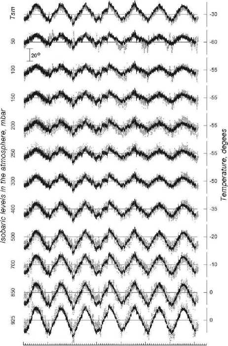
The results thus obtained are shown in Figure 6. The atmospheric temperature variations in isobars found from the data on muon intensity variations are shown by the solid line. Dots mark direct measurements — aerological sounding data from the weather station Bugrinskaya Roshcha (Novosibirsk). The weather station is located at about 35-40 km from a CR station. Sounders were launched twice a day. On the left are isobars representing the temperature measurements; on the right is the average temperature in the isobar. The scale of temperature variations is the same for all the isobars (top). At the top are variations of the weight average (average by weight) atmospheric temperature (WAT) for the entire period nn

A T_c = E A T_r A h , /EA h .                  (11)

i = 1                   i = 1

Here Δ T i is the layer temperature variations (isobars) i , Δ h i is the mass of this layer.

The results are in satisfactory agreement with the direct measurements for all seasons. Slightly worse agreement is observed for the winter period. This is attributed, on the one hand, to the fact that the temperature variations on the isobars are found as deviations from annual average vertical temperature distribution, which almost coincides with the vertical distribution of the average temperature for spring and fall (this reduces computational errors). On the other hand, the worst agreement between the results for the winter period is due to the low quality of aerological sounding data when the sharply increasing number of gaps in measurements is statistically significant. The presented direct measurements (aerological sounding data) for these periods are often the result of extrapolation. Further improvement of the method requires a more careful approach to the formation of the sample (length and quality of direct measurements) and to the evaluation of temperature coefficient density distribution for atmospheric muons (weight function).

2004    2005    2006    2007    2008    2000    2010    2011

Years

Figure 6. Atmospheric temperature variations at different isobaric levels: calculation result (solid line), aerological sounding data (dots)

CONCLUSION

Thus, continuous observations of CR intensity variations made at CR stations equipped with muon tele- scopes will provide information about vertical atmospheric temperature distribution in real time. The accuracy of this information will depend on the number of channels of muon detection at different zenith angles. For a more accurate description of the vertical atmospheric temperature distribution we should use the sixth degree polynomial, which will require at least seven directions of muon detection at different zenith angles. If there are only five channels of muon detection, the problem is solved but with the fourth degree polynomial. The result will, however, be rougher.

The work is based on data from the Unique Research Facility URF-85 “Russian National Network of Cosmic-Ray Stations”.

This work was performed with budgetary funding of Basic Research program No. 0331-2019-0013 "Manifestation of processes of the deep geodynamics in geospheres as derived from monitoring of the geomagnetic field, ionosphere, and cosmic rays".