Variation Level Set Method for Multiphase Image Classification

Published Online August 2011 in MECS

The objective of this work is image classification that is a basic problem in image processing. Although this task is usually easy and natural for human beings, it is difficult for computers. Image classification is considered as assigning a label to each pixel of an image. A set of pixels with the same label represent a class. The purpose of classification is to get a partition compound of homogeneous regions. The feature criterion is the spatial distribution of intensity. Stochastic approach was first proposed in [1]. Later a supervised variational classification model based on Cahn-Hilliard models was introduced in [2]. During recent years many classification models have been developed to improve the quality of image classification ([3], [4], [5], [6]).

Osher and Sethian [7] proposed an effective implicit representation called level set for evolving curves and surfaces, which allows for automatic change of topology, such as merging and breaking. A supervised mode based on level set and region growing method was developed in

• [8] . However, this model doesn’t include the estimation for the intensity values of each region and level set function needs to be re-initialized. To solve these problems, an unsupervised model is proposed in this paper. Li [9] firstly introduced a level set evolution without re-initialization. In this paper a similar term is introduced to improve our model. The new term can force the level set function to be close to a signed distance function.

In the classification process the information is often neglected that is the orientation of the image gradients. The gradient magnitude edge indicator is not enough for capturing thin structures. Vasilevskiy and Siddiqi used maximization of the inner product between a vector field and the surface normal in order to construct an evolution that is used for segmentation of thin structures [10]. This term is a reliable edge indicator for relatively low noise levels. In the case, high noise levels, additional regularization techniques are required.

The resulting of the proposed model is a set of Partial Differential Equations. These equations govern the evolution of the interfaces to a regularized partition. The evolution of each interface is guided by forces which include internal force based on regularization term, external force based on region partition term and boundary alignment term. The term of re-initialization is used to penalize the deviation of the level set function from a signed distance function.

This paper is organized as follows. First, the problem of classification is stated as a partition problem. Then Set the framework and define the properties about classification. Second, an unsupervised classification model based on level set evolution is proposed through a level set formulation. The Euler-Lagrange derivative of the model leads to a dynamical equation. Finally, some experiment with promising results are presented.

• II.    IMAGE CLASSIFICATION FRAMEWORKS

In this section the properties which the classification model needs to satisfy with are presented. The classification of the problem is considered as a partition problem. Each partition is compound of homogeneous region are unknown and should be estimated before classification. In next section the estimation method of intensity values will be discussed in detail. In order to complete classification some feature criterions should been defined.

Let Q be an open domain subset of R ², with 5Q its boundary. Let C be a closed subset in Q , made up of a finite set of smooth curves. The connected components of Q C ^are denoted by Q_t , such that Q = U, Q U C • Let

Uо : Q ^ R represents the image intensity. Each region in the image is characterized by its mean intensity (u i )i =123 k . The number K of total phases is supposed to be given from a previous estimation. And let Qi be the region defined as

Q i = { x gQ| x g Ui } .              (2)

A partitioning which penalizes overlapping and the formation of vacuum is considered to find a set {q.}. =1    k , where

k

Q = U Q i and Q i I Q j =0 .     (3)

i = 1                   i * j

In the next section the solution of classification model has to take into account these conditions.

• III.    multiphase classification model

The unsupervised model in this paper is inspired by the work ([7], [8], [9]). In this paper we use a level set formulation to represent each interface and region. In this paper we use a level set formulation to represent each interface and region.

A. Preliminaries Let ф. : Q x R + ^ R be a Lipschitz function associated to region Qi ф, (x, t )> 0 fx g Q ф( x,t ) = 0 fx g 6Qi . (4) ф( x,t )< 0 fx g otherwise regions separated by interfaces. Herein, suppose that each class has a homogeneous distribution of intensify (or grey level). Therefore each class is characterized by its mean value of grey level. However, the intensity values of each

Thus the function ф . ( x , t )

is used to describe the

region Q i and dQ i represents the boundary of Q i . In the following, we will sometimes omit spatial parameter

• x and time parameter in ф . ( x , t ) .

B.    Parameters Estimation

In order to complete partition region, the estimation for the intensity values of each region in and insure the computation of a global minimum, let we define the approximations H^ and §а of Heaviside and Dirac functions, as shown in Fig 1(a) and Fig 1(b).

<

^H а ( Ф ) = 2 [ 1 +

2 arctan

П

⁵“ ( ф ) = ¹ (., п V а + ф

The estimation for the intensity values of each region should be done because these parameters in this model are unknown before classification. In this paper, We use mean intensity values of each region as parameters. So the parameter estimation can be completed by following formulation

J ^U 0 * ^H а ( Ф )

U = ■^Q—T------7 7•

' J ^H а ( Ф . )

Q the

C.    Class f cat on Funct ons n Term of Level Set

The partition {Qi}        based on the level set can be achieved through the minimization of a global function. This global function contains four terms. In the following, each term will be expressed.

Let define the first function related to (3)

k ²

F C = 7 J_Q I H а ( Ф ) - 1 dxdy. (7)

²     V i = 1                 2

The minimization of F ^ penalizes the formation of vacuum and region overlapping.

The second function is related to external force and takes into account the parameter estimation.

k ₂

F^e = I e, J H ( ф )( U_o - U i ) dxdy , e i g R , V i (8)

i = 1     Q

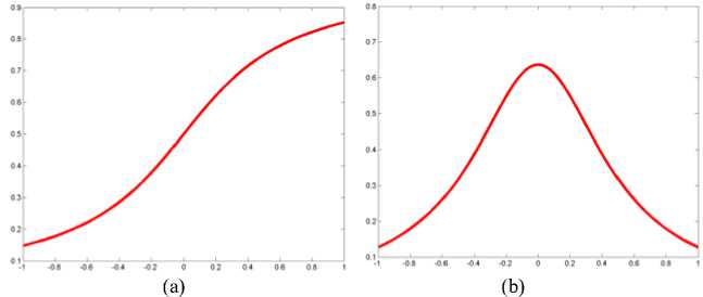
Fig.1 Regularized versions of the Heaviside function and. 5 function ( a = 0.5 ). (a) The regularized versions of the Heaviside function. (b) Regularized versions of 5 function.

We define parameters u_i as

J “ 0 * ^H a ( ^ф )

J ^H . ( Ф 1 )

Q

^U L

= u L2 + U L2 + 2u LL xx 1yy 2xy 12

The third term in our model is related to boundary

alignment. Zero crossing of the second order derivative along the gradient direction is introduced. And then he . observed that using only the gradient direction

U^V “ I J

component of the Laplacian yields better edges than those produced by the zero crossing of the Laplacian.

So the curve evolves along the second order derivative in the direction of the image gradient. Then the boundary alignment term in our model is described as below

F^b = J A u -|V u| V-

Q

V u

M

. H ( ф ) dxdy

where u represents a gray level image. Let

define _u ( x , y ): R ² ^ [ 0,1 ] . The first order derivatives in the

horizontal and vertical directions are represented by

u and u , respectively. We define the gradient direction xy

vector field

; = 2 “ = ^{ “ ■ u y ^}

I^V “\     “x² + “y ²

and the orthogonal vector filed r   VU    {— “y , “x } n = — = I      .

I^{V U} l   V “x ^{2 +} uy²

denotes inner product of

two vectors. The edge detector finds the image locations where both V U is larger than some threshold

and u ^ = 0 , where “ ^ is the second derivative of ^u in the gradient direction. Then we can get the description of “ l as below

This term is important for finding edges of thin structures in images. However, this term alone is insufficient for integrating all the edges. If the curve used as an initial guess is far from the object boundaries, it may fail to lock onto its edges. Therefore, another ‘force’ that pushes curve toward the edges of the object is required.

The fourth function that we want to introduce is related to internal force about minimization of the interfaces length

k

F¹ = ^ Y i J 5 (^ ф. ) | V ф _i \, у. e R, Vz . (14) i =1 Q

The last function in this model is related to reinitialization. It is crucial to keep the level set function as an approximate signed distance function during the evolution. The standard re-initialization method is to solve the following equation

^d ^= sign ( ^ф 0 ) ( 1 -|^{v ф} )

where ф ₀ is the function to be re-initialized, and

sign ( ф ₀ ) is the sign function. However, if ф ₀ is not smooth or much steeper on one side of the interface than the other, the zero level set function ф can be moved incorrectly. In this paper, we introduce a new term that forces the level set function to be close to a signed distance function, and therefore completely eliminates the need of the costly re-initialization procedure. The term is described as below

k ₂

F' ™ = Z M A - ( V ф^- 1 ) dxdy .     (16)

‘ =¹      П ²

By minimizing (11), the corresponding partial differential equations of ф is given by

^{д ф} = А ф - V ■ d t

" V ф 1Й J

The Euler Lagrange equations associated to F _a can be achieved by minimizing the above global function F _a . And then through it embedding into a dynamical scheme by using the steepest descent method, we can get a set of equations

д ф

— = ц . ^Аф . ^{- V} ■ d t

I ^V Ф I

^ф ( 0, x , y ) = ^ф о ( x , y )

- 5

: uo - u ^² )

To explain the effect of the term, we notice that the gradient flow

- y . * 5 ( ф. ) * V ■

= V. 1 -

N г.

has the factor f 1 1 ) as diffusion rate. If Vф > 1, the V -n J diffusion rate is positive. It will make ф more even and therefore reduce the gradient V ф . If V ф < 1, the term

has effect of reverse diffusion and therefore increase the gradient.

We use an example, as shown in Fig 2 to explain the effect of this term. From the result we can see that even though the initial level set function in Fig 2(a) is not a signed distance function the evolving level set function, as shown in Fig 2(b), is maintained very close to a signed distance function. The result of evolution is represented in Fig 2(c)

Thus taking into account the parameter estimation, the sum F^cF^eF F ⁿ F^b leads to the global function

F = F C + F^e + F‘ + F™ + F^bu

У ф , I^V Ф I

+ ²⁵ ( ^ ) J Z ^h ( ф ) - ¹

n V ' = 1

- 5 ( ф , ) А u , -|V u jV.

V u

o

I^{V u}o|

.

Thus the numerical algorithms of (20) can be written

as

■^{1 1 1} = ^ф - ^dt * ⁵ ( ф ) ( е ( ^uo ^{- u}d )

+ dt * 5 ( ф ) * у . *V ■

Vфl

I V i l

+ dt * 25 ( ф ) J Z H ( ф .) - 1

+ dt * 5 ( ф ) A u_o -|V u_o | V.

V u

o

I ^{V u}o|

.

2            ^

• +- J Z H ( ф )^{- 1} 1 dxdy

• ² qV= 1          J

k ₂

⁺ Z e . J_n H ( ^ф )( ^u o ^- u . ) dxdy

I = 1

k

⁺ Z ² J , ^ ( ф ) ^V ф|^dxdУ

= 1

• ^k 1               2

• ⁺Z ^ -J^W^{- 1} ) dxdy

I = 1        ²

k

⁺ ZJ ^{A u} o -N ^V

■ =1 Ш

V u

o

I ^{V u} o\

* H ( ф ) dxdy .

D. Evolut on and Numer cal Scheme

• IV.    experimental results

In this section we conclude this paper by presenting numerical results using our model on various synthetic and real images. In our numerical experiments, we general choose the parameters as follows: h = 1 (the step space), А t = 1 (the time step). We use the approximations H _a and 5_a of Heaviside and Dirac functions ( O =Q 5 ). These results show our model can complete the classification and get the better result although the parameters are unknown. The model also avoids the re-initialization in level set evolution.

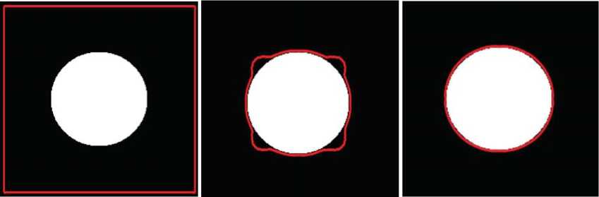
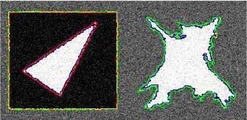
Fig.3 shows experiment on a synthetic image with three classes. In this experiment we use three level set functions. In Fig.3 (a) it is the result based on model without boundary alignment term. Fig.3 (b) is the result of our method. From the result it shows that although our method needn’t know parameters before classification it can complete the classification tasks. So it can save much work to identify region parameters and get the better result, especially for dealing with the edge of square, by using the new boundary alignment term.

(a)                       (b)                            (c)

Fig.2 : Evolution of level set function to explain the re-initialization term. (a) The initialization of level set function. (b) The evolution of level set function. (c) The result of evolution.

(a)

(b)

Fig.3 Classification for synthetic image based on parameters estimated method. (a) The result of the model without boundary alignment term. (b) The result based on our method. Parameters in the model are respectively:

Y ₁ = Y 2 = Y 3 = 3 * 255 * 255, ^e 1 = ^e 2 = e 3 = 10, ^ = 4 * 10 4 , M 1 = М 2 = М 3 = 5 * 10 - 2 .

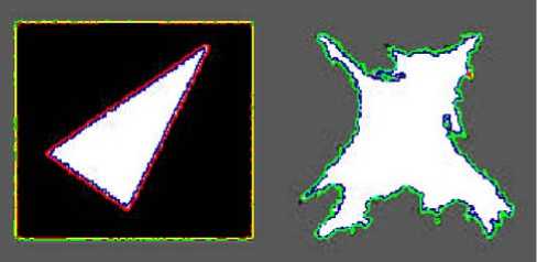
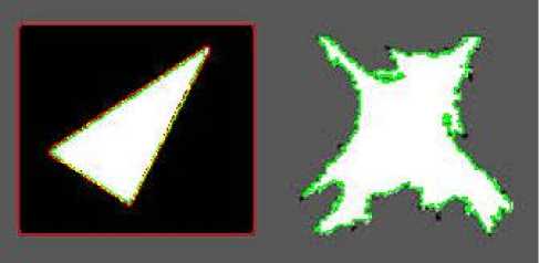
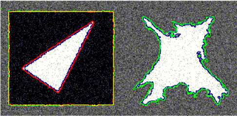
In Fig.4, we show how our model works on a gauss noise image with three classes. In this experiment we use three level set functions. This noise picture is done by us. Fig.4 (a) shows the result based on model without boundary alignment term. In Fig.4 (b) we show the result of classification based on our method. From the result it shows that although the image has noise our model can complete the classification tasks and get the better result, especially for dealing with the edges of three shapes.

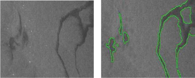
In Fig.5 it shows the experiment on an oil spills image with blurred boundaries. Spillage of oil in coastal waters can be a catastrophic event. The potential damage to the environment requires agencies to rapidly detect and clean up any large spill. In this experiment we use two level set functions. In Fig.5 (a) we show the original picture. In Fig.5 (b) we show the result of classification based on our model. The result shows that this model can rapidly discriminate oil spills from the surrounding water

In Fig.6 we show the experiment on a medical image. This image is a 2D MR brain image with structures of different intensities and with blurred boundaries.

(a)

(b)

Fig.4. Classification for a gauss noise image. (a) The result of the model without boundary alignment term. (b) The result of classification based on our model. Parameters in the model are respectively:

Y 1 = Y 2 = Y ₃ = 3 * 255 * 255, e 1 = e ₂ = e 3 = 10, X = 4 * 10⁴, Ц 1 = Ц 2 = Ц 3 = 5 * 10 ².

(a)                                         (b)

Fig.5. Classification for an oil spill image. (a) The origin image. (b) The result of classification based on our method. Parameters are respectively:

Y 1 = y ₂ = 0.5 * 255 * 255, e 1 = e 2 = 100, X = 4 * 10⁴, ц 1 = ц ₂ = 5 * 10 ^{- 4}.

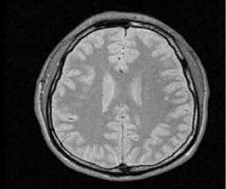
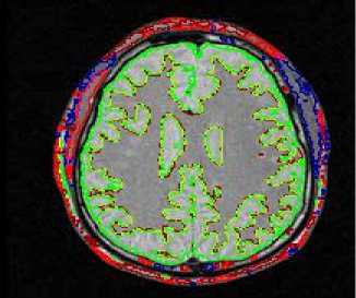
Fig.6. Classification for a medical image. (a).The origin image. (b) The result of classification based on our method. Parameters in the model are respectively :

Y i = Y ₂ = Y 3 = 3 * 255 * 255, X = 4 * 10⁴, e 1 = e ₂ = e ₃ = 10,

In this experiment we use three level set functions. Fig.6 (a) shows the origin picture. Fig.6 (b) is the result of classification based on parameters estimation. The result shows that our model can force the curves to converge on the desired boundaries even though some parts of the boundaries are too blurred.

• V.    Conclusions

  • [8]    C. Samson, L.Blanc-Féraud, G.Aubert, and J.Zerubia, “A Level Set Model for Image Classification,” Int. J. Comput. Vis , vol. 40, pp. 187–197, 2000.

  • [9]    C. Li, C. Xu, C. Gui and D.Martin, “Level set Evolution Without Reinitialization: A New Variontional Fomulation,” IEEE Int Conf. Comput. Vis. Pattern Recognit., San Diego, vol.1, pp.430-436, 2005.

  • [10]    A. Vasilevskiy and K. Siddiqi, “Flux maximizing geometric flows,” IEEE Trans. Pattern Anal. Machine Intell., vol. 24, pp. 1565– 1578, 2002.

In this paper an unsupervised classification model based on level set is proposed. This new model has parameters estimation capability. Parameter estimation is automatically completed in classification process. This model also include a new term that forces the level set function to be close to a signed distance function So it eliminates the need of the re-initialization of level set function. In addition, a boundary alignment term is also included in this model that is used for segmentation of thin structures. The resulting of this new model is a set of Partial Differential Equations. These equations govern the evolution of the interfaces to a regularized partition, even if the original image is noisy and has the structures with blurred boundaries. Finally this proposed model has been applied to both synthetic and real images with promising results. However, this new model only uses the spatial distribution of intensity. So this new model needs to be improved incorporating with other features of the image.

Zhong-Wei Li, born in 1979. He is currently a Ph. D degree candidate in college of physics science at Graduate University of Chinese Academy of Science, Beijing. His research interests include differential equations, medical simulation and image processing.

Acknowledgment

This work was supported by the National Natural Science Foundation of China (Grant No.50936006).