Very Large Scale Optical Interconnect Systems For Different Types of Optical Interconnection Networks

Numerous applications for interconnection networks with extremely high throughput and low latency have been studied previously, including high-performance computing and telecommunications core routing [1]. Optical interconnection networks (OINs) are able to meet many of these system requirements by leveraging the large bandwidth afforded by fiber-optic and photonic technologies. Multiple stage (or multistage) interconnection networks (MINs) offer topological advantages such as scalability and modularity owing to their composition from hundreds or thousands of similar switching node building blocks [2]. In OIN systems, most of the complexity and cost is attributable to the photonic switching elements. When multiple wavelength data is employed, these switching elements must execute space switching in addition to wavelength switching. Many switching node designs based on this technique have been proposed and most are implemented with semiconductor optical amplifier (SOA) switching gates. The effectiveness of parallel computers is often determined by its communication network. The interconnection network is an important component of a parallel processing system. A good interconnection network should have less topological network cost and keep the network diameter as shorter as possible [3].

In the present study, an important issues in the design of optical interconnection networks for high performance computing and communication systems is scalability. As well as different types of optical interconnection networks for scalable high performance communication and computing systems have been modeled, investigated and a analyzed numerically and parametrically over wide range of the affecting parameters. Optical interconnection networks is a promising design and performance parameters alternative for future systems. Numerous configurations with different degrees of optics, optoelectronics, network diameter, node degree, bisection width, scalability, transmission capacity, cost evolution, and electronics have been proposed.

II.    Current Architectures for Scalable Parallel Computing Systems

II.    1. Scalable optical crossbar connected interconnection network (SCON)

SOCN stands for “scalable optical crossbar connected interconnection Network”. A two-level hierarchical network. The lowest level consists of clusters of n processors connected via local WDM intra-cluster all-optical crossbar subnetwork. Multiple (c) clusters are connected via similar WDM intra-cluster all-optical crossbar that connects all processors in a single cluster to all processors in a remote cluster. The inter-cluster crossbar connections can be rearranged to form various network topologies [5].

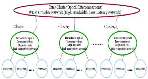
Fig. 1. Scalable optical crossbar connected interconnection network [6].

Both the intra-cluster and inter-cluster subnetworks are WDM-based optical crossbar interconnects. Architecture based on wavelength reuse. The SOCN class of networks are based on WDM all-optical crossbar networks. The benefits of crossbar networks are fully connected, minimum potential latency, highest potential bisection bandwidth, can be used as a basis for multistage and hierarchical networks. But disadvantages of crossbar networks are O (N2) complexity, difficult to implement in electronics, N2 wires and switches required, rise time and timing skew become a limitation for large crossbar interconnects, optics and WDM can be used to implement a crossbar with O (N) complexity [6].

II.    1. 1. Optical crossbar connected cluster network (OC3N)

Every cluster is connected to every other cluster via a single send/receive optical fiber pair. Each optical fiber pair supports a wavelength division multiplexed fully-connected crossbar interconnect. Full connectivity is provided: every processor in the system is directly connected to every other processor with a relatively simple design. Inter-cluster bandwidth and latencies similar to intra-cluster bandwidth and latencies. Far fewer connections are required compared to a traditional crossbar [7].

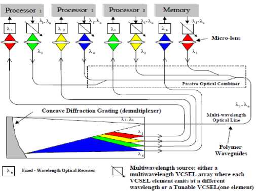
Fig. 2. WDM optical crossbar implementation [7].

Each processor contains a single integrated tunable vertical cavity surface emitting laser (VCSEL) or a VCSEL array, and one optical receiver. Each VCSEL is coupled into a personal board integrated polymer waveguide. The waveguides from all processors in a cluster are routed to a polymer waveguide based optical binary tree combiner. The combined optical signal is routed to a free space diffraction grating based optical demultiplexer. The demultiplexed optical signals are routed back to the appropriate processors [7]. The OC3N topology efficiently utilizes wavelength division multiplexing throughout the network, so it could be used to construct relatively large (hundreds of processors) fully connected networks with a reasonable cost. One of the advantages of a hierarchical network architecture is that the various topological layers typically can be interchanged without effecting the other layers. The lowest level of the SOCN is a fully connected crossbar. The second (and highest) level can be interchanged with various alternative topologies as long as the degree of the topology is less than or equal to the cluster node degree are crossbar, hypercube, tree, and ring [8].

II.    1. 2. Optical hypercube connected cluster network (OHC2N)

Processors within a cluster are connected via a local intra-cluster WDM optical crossbar. Clusters are connected via inter-cluster WDM optical links. Each processor in a cluster has full connectivity to all processors in directly connected clusters. The intercluster crossbar connecting clusters are arranged in a hypercube configuration [9].

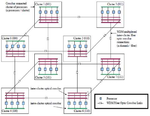
Fig. 3. Optical hypercube connected cluster network [9].

The OHC2N does not impose a fully connected topology, but efficient use of WDM allows construction of very large-scale (thousands of processors) networks at a reasonable cost [9].

III.    Theoretical Model Analysis

III.    1. Performance parameters of OC3N and OHC2N networks

III.    1. 1. Diameter and link complexity

The diameter of the network is defined as the maximum distance between two any processors in the network. Also defined as For each possible pair of nodes in the network there exist a shortest path. The diameter is defined as the number of hops over the longest of these shortest paths [7]. The number of nodes for different networks (OC3N and OHC2N) are:

NC = nxc , for (OC3N network)(1)

NH = nx 2d , for (OHC2N network)(2)

Where n is the number of processors per cluster, c is the number of clusters, d is the network diameter and is:

d = unity , for (OC3N network)(3)

( N 1

d = log ₂ 1 I , for (OHC 2 N network) I n )

Where the link complexity or node degree is defined as the number of physical links per node. Also can be defined as the number of links that connects a node to its nearest neighbors. The node degree can either be constant for the whole network or differ between the nodes [8]. Where the node degree K for different networks ( OC³N and OHC²N) are:

N

K = c = — , for (OC³N network)          (5)

n

K = d + 1, for (OHC 2 N network)          (6)

III.    1. 2. Bisection bandwidth

The bisection of a system is the section that divides the system into two halves with equal number of nodes. The bisection bandwidth is the aggregated bandwidth over the links that cross the bisection. In asymmetric systems the number of links across the bisection depends on where the bisection is drawn. However, since the bisection bandwidth is a worst case metric, the bisection leading to the smallest bisection bandwidth should be chosen [9]. Where the number of links L for different networks (OC3N and OHC2N) are given by:

L C = 0.5 J N ² - N | , for (OC³N network)       (7)

I n ²      n J

L H = 12 ^dd = N log₂ — , for (OHC 2 N network) (8) 2       2 n n

In the same way, the bisection bandwidth for different networks ( OC³N and OHC²N) are given by [11]:

B w c = N 42 = I nxc ² , for (OC³N network)     (9)

BW H = n 2 ^{d - 1} = N , for (OHC 2 N network)      (10)

III.    1. 3. Average message distance

The average message distance in the network is defined as the average number of the links that a message should travel between any nodes. Let N i is the number of nodes at distance i, then the average distance l is defined as [12]:

n l=N-1 i      •

Therefore the average message distance for different networks (OC3N and OHC2N) are given by [11, 12]:

IC = unity , for (OC3N network)(12)

H =       0.5 N log 2 ( N ¹ + ( n - 1 ) , (OHC²)

N -1 L|

III.    1. 4. Cost scalability of different networks

A major advantage of a SOCN architecture is the reduced hardware part count compared to more traditional network topologies. The cost scalability of the two networks can be estimated based on the number of the tunable VCSELs V, number of detectors per processor D, and waveguides per processor W, and number of demultiplexers in the cluster M as:

Cost C = nV + nD + nW + cM ,$ for(OC³Nnetwork) (14) Cost H = log ₂ ( nV + nD + nW + cM ), $ for (OHC 2 N network) (15)

III.    1. 5. Transmission capacity of different

NETWORKS

The transmission capacity per subscriber (C T ) can be expressed in terms of number of quantization levels (Q), and the actual bandwidth for audio signal bandwidth (B.W _A ) for different interconnection network as [13]:

C t ( Audio ) = B W ac log 2 Q , for (OC³N network)    (16)

C t ( Audio ) = B W ah log 2 Q , for (OHC 2 N network) (17) Where B.W AC is the multiplication of the bandwidth of audio signal (around 3.4 KHz-4 KHz) and the bisection bandwidth for optical crossbar connected cluster network (OC³N), and also B.W AH is the multiplication of the bandwidth of audio signal and the bisection bandwidth of optical hypercube connected cluster network (OHC²N). In the same way, The transmission capacity per subscriber (C _T ) can be expressed in terms of number of quantization levels (Q), and the actual bandwidth for audio signal bandwidth (B.W A ) for different interconnection network as follows [14]:

C t ( Video ) = B W vc log 2 Q , for (OC 3 N network)    (18)

C t ( Video ) = B W vh log 2 Q , for (OHC 2 N network) (19) Where B.W VC is the multiplication of the bandwidth of video signal (around 6.8 MHz-8 MHz) and the bisection bandwidth for optical crossbar connected cluster network (OC³N), and also B.W VH is the multiplication of the bandwidth of video signal and the bisection bandwidth of optical hypercube connected cluster network (OHC²N).

IV.    Simulation Results and Discussions

We have analyzed parametrically, and numerically the have been modeled, investigated and a analyzed numerically and parametrically over wide range of the affecting parameters optical interconnection networks are a promising design and performance parameters alternative for future systems. Numerous configurations with different degrees of optics, optoelectronics, network diameter, node degree, bisection width, scalability, transmission capacity, and cost evolution,. Based on the modeling equations analysis and the assumed set of the operating parameters as shown in Table 1.

Table 1: Proposed operating parameters for optical interconnection network model.

Operating parameter	Definition	Value and units
B.W A	Bandwidth of the audio signal	3.4 KHz ≤ B.W A ≤ 4 KHz
B.W V	Bandwidth of the video signal	6.8 MHz ≤ B.W V ≤ 8 MHz
Q	Number of quantization levels	16 ≤ Q ≤ 1024
V	Number of tunable VCSELs/processor	10 ≤ V ≤ 100
D	Number of detectors/processor	10 ≤ D ≤ 100
W	Number of waveguides/processor	10 ≤ W ≤ 100
M	Number of demultiplexers/cluster	10 ≤ M ≤ 100
c	Number of clusters	16 ≤ c ≤ 128
n	Number of processors/cluster	16 ≤ n ≤ 128
N	Number of nodes or processors	64 ≤ N ≤ 1024
d	Network diameter	1 ≤ d ≤ 15

The following facts are assured as shown in the series of Figs. (4-29):

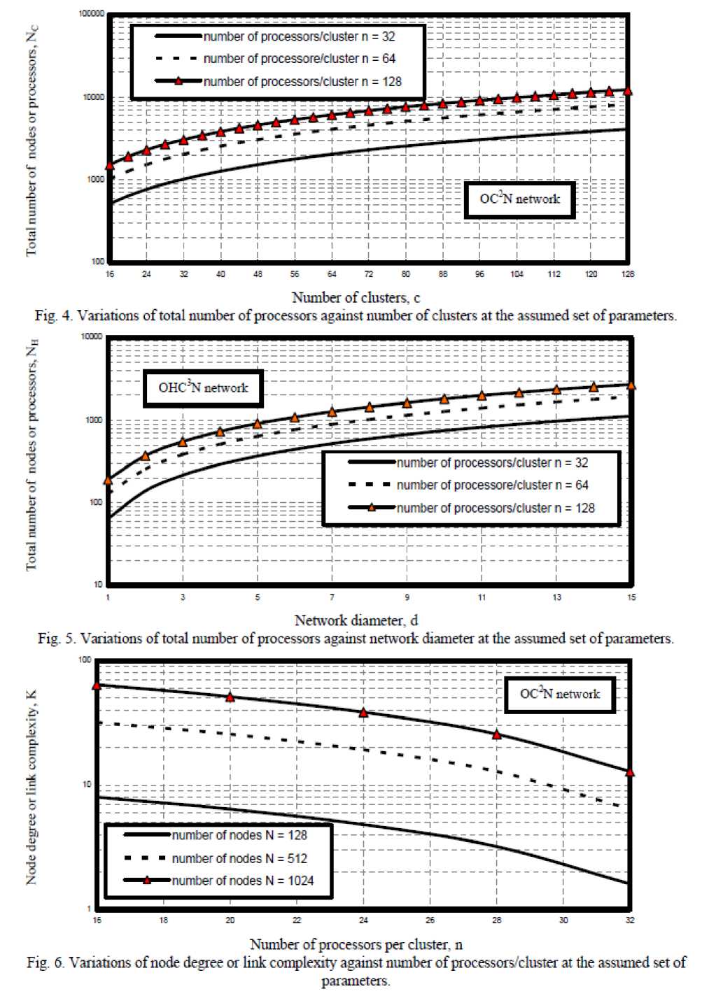
• i)    As shown in Fig. 4 has indicated that as both number of clusters and number of processors per cluster increase this lead to increase in total number of nodes or processors in the case of optical crossbar connected cluster network.

• ii)    Fig. 5 has assured that as both number of processors per cluster and network diameter increase this lead to increase in total number of nodes or processors in the case of optical hypercube connected cluster network.

• iii)    As shown in Fig. 6 has indicated that as both number of processors and number of processors per cluster increase this lead to increase in node degree or link complexity in the case of optical crossbar connected cluster network.

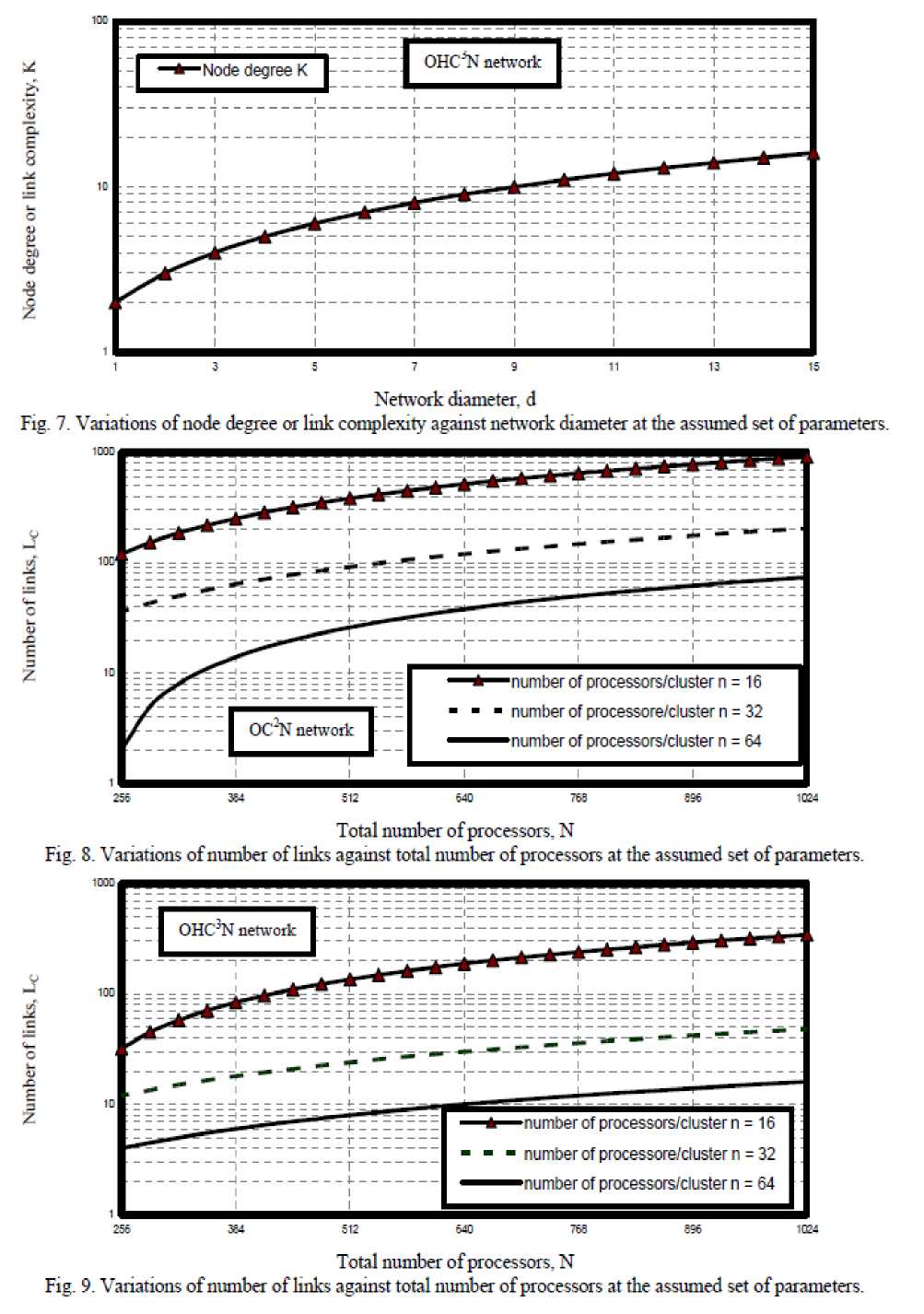
• iv)    Fig. 7 has assured that as network diameter increase this leads to increase in node degree or link complexity the case of optical hypercube connected cluster network.

• v)    Figs. (8, 9) have demonstrated that as total number of processors increase and number of processors per cluster decrease this lead to increase in number of links as in the case of both optical crossbar connected cluster and optical hypercube connected cluster networks. We

observed that number of links in optical crossbar connected cluster network is larger than optical hypercube connected cluster network.

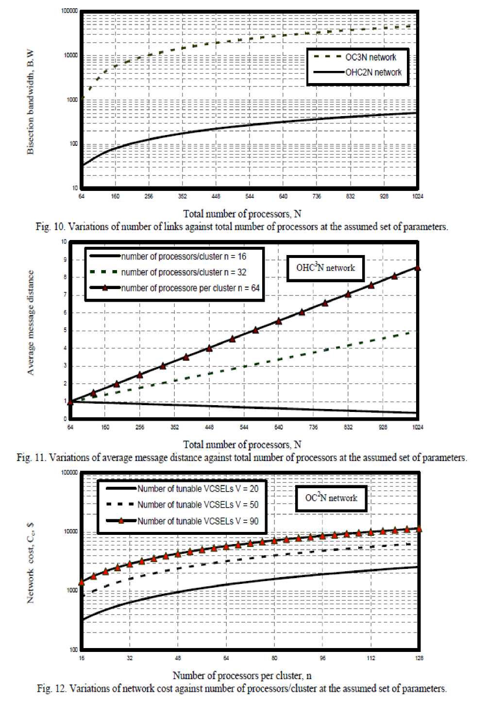
• vi)    As shown in Fig. 10 has proved that as total number of processors increase, this result in increasing bisection bandwidth in both optical crossbar connected cluster and optical hypercube connected cluster networks.

• vii)    As shown in Fig. 11 has demonstrated that as both number of processors per clusters and total number of processors increase, this result in increasing average message distance in the case of optical hypercube connected cluster network but average message distance equal to unity in the case of optical crossbar connected cluster network.

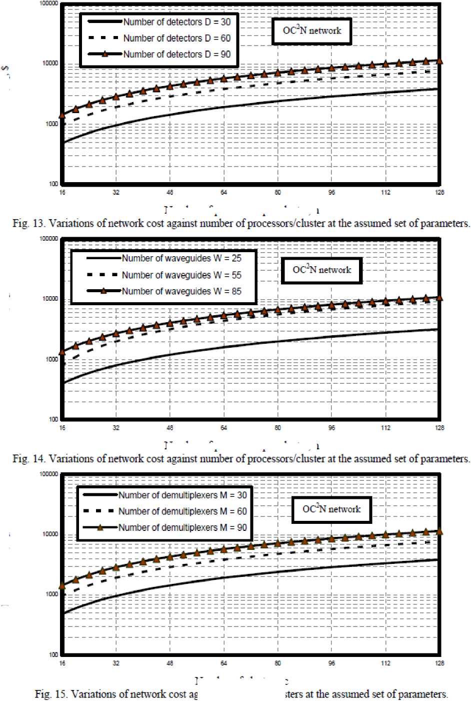
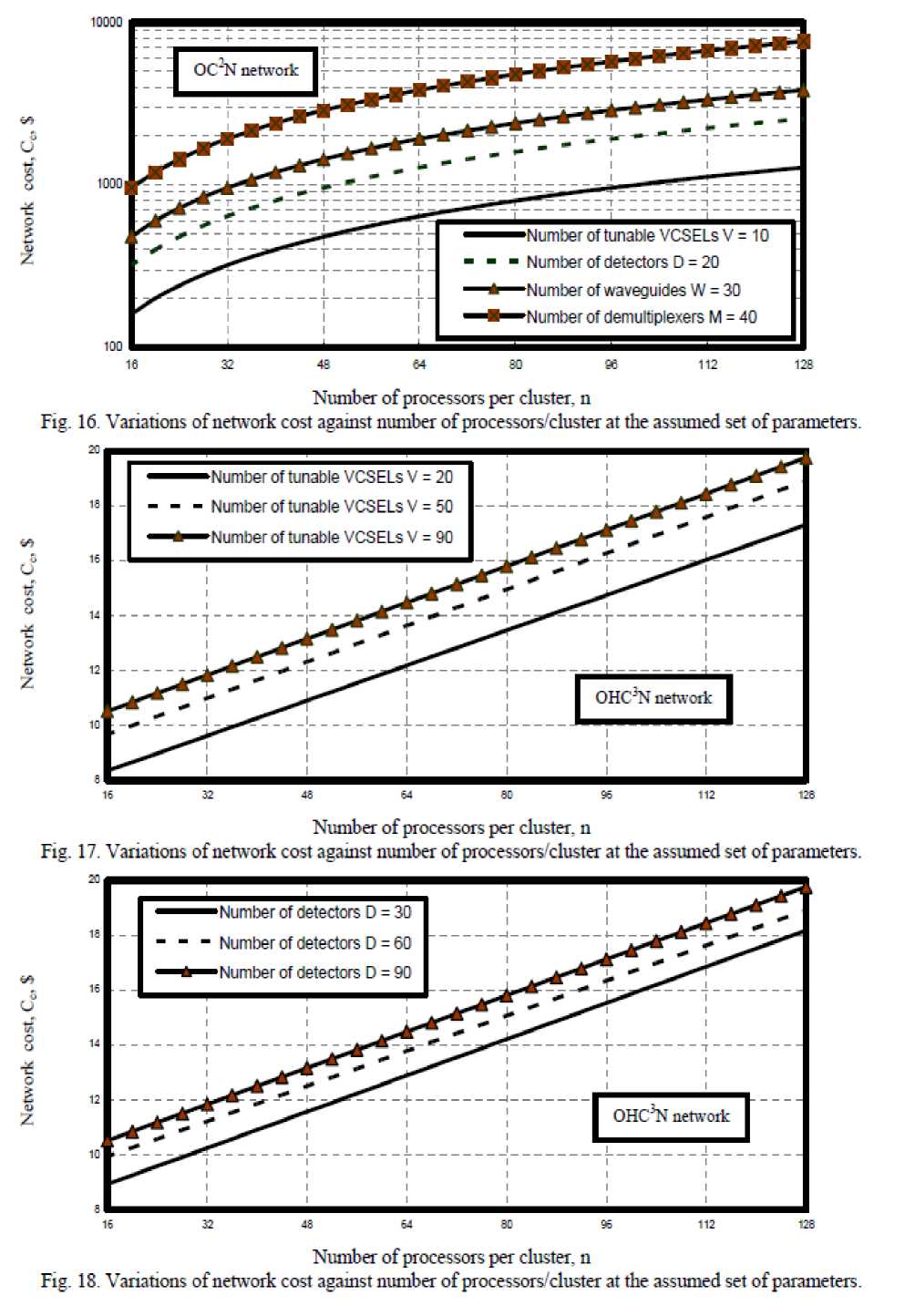
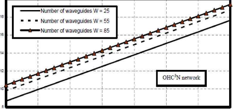
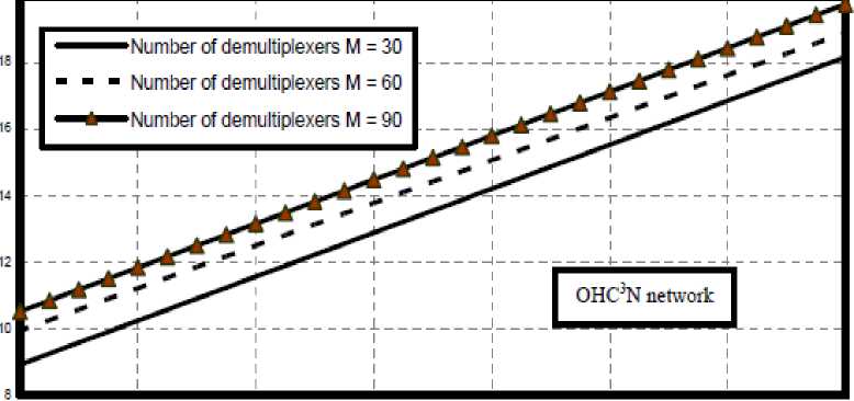
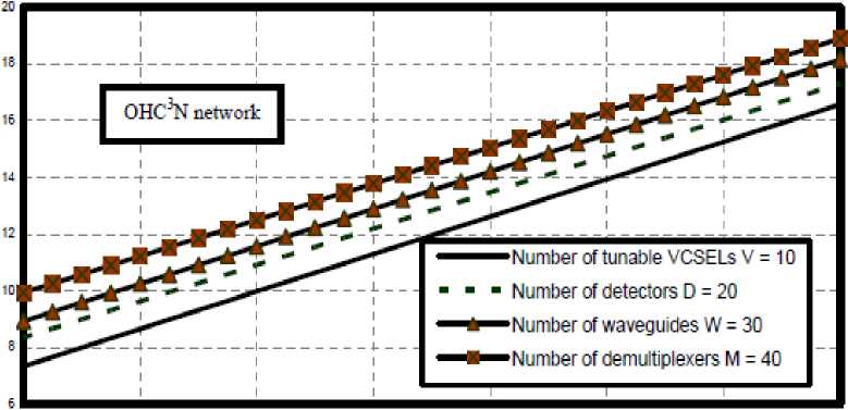
viii) Figs. (12-21) have assured that as number of processors per cluster, number of tunable VCSELs, number of detectors, number of waveguides, number of demultiplexers, and number of clusters increase this result in increasing in network cost in the case of both optical crossbar connected cluster and optical hypercube connected cluster networks. We have indicated that optical crossbar connected cluster network is higher network cost than optical hypercube connected cluster network.

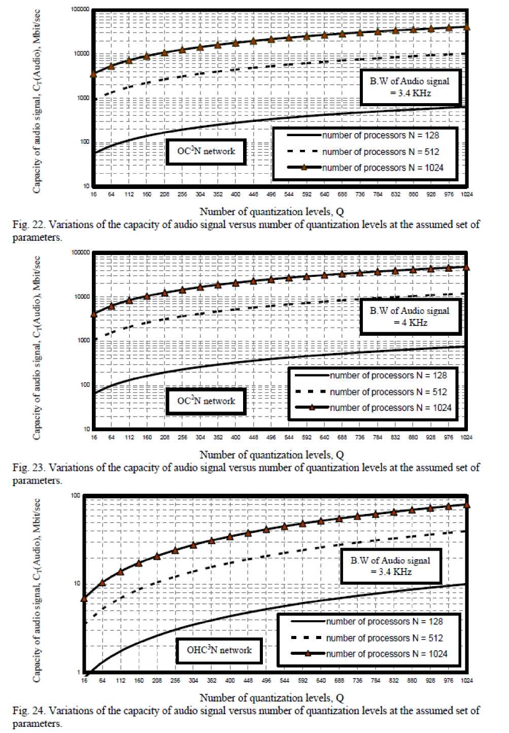
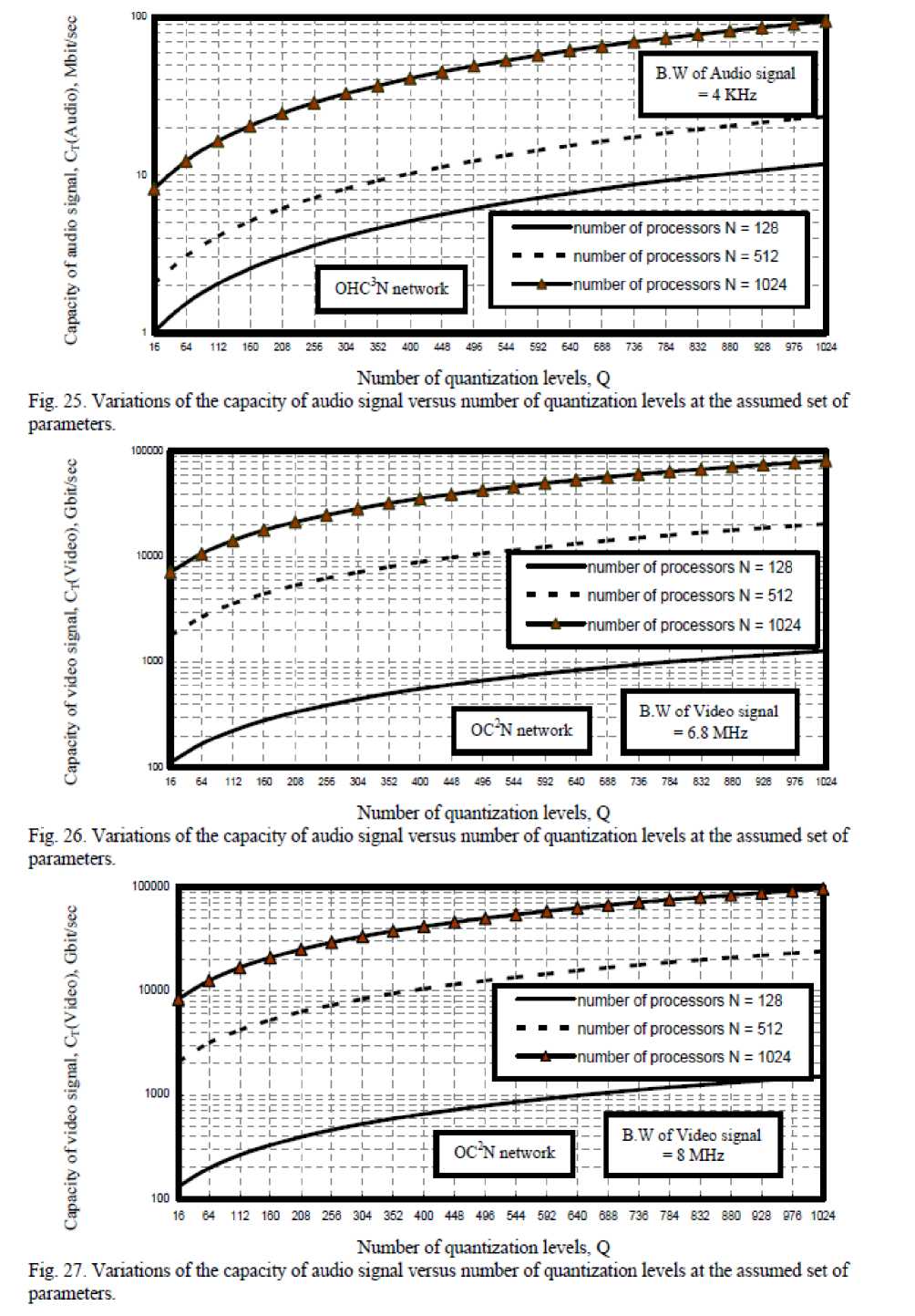
• ix)    As shown in Figs. (22-25) have indicated that as number of quantization levels, number of processors and bandwidth of audio signal increase, this lead to increase in the transmission capacity of bit rates for both crossbar connected cluster and optical hypercube connected cluster networks. We have observed that optical crossbar connected cluster network is higher transmission bit rates than optical hypercube connected cluster network.

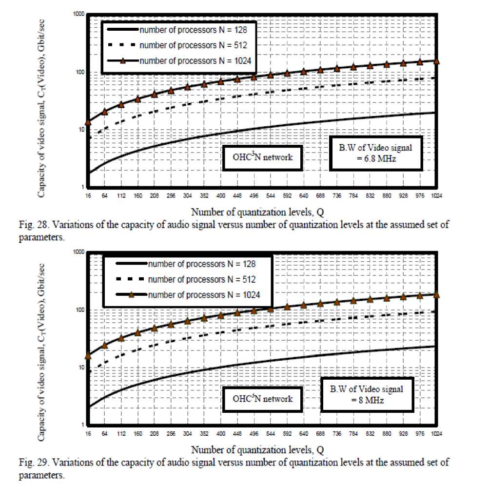
• x)    As shown in Figs. (26-29) have indicated that as number of quantization levels, number of processors and bandwidth of video signal increase, this lead to increase in the transmission capacity of bit rates for both crossbar connected cluster and optical hypercube connected cluster networks. We have observed that optical crossbar connected cluster network is higher transmission bit rates than optical hypercube connected cluster network.

•сох

100С

1ХОХ

Number of processors per cluster, n

Fig. 6. Variations of node degree or link complexity against number of processors/cluster at die assumed set of parameters.

Number of clusters, c

Fig. 4. Variations of total number of processors against number of clusters at the assumed set of parameters.

1O00C

100C

OC~N network number of nodes N = 128

number of nodes N = 512

number of nodes N = 1024

Network diameter, d

Fig. 5. Variations of total number of processors against network diameter at die assumed set of parameters.

OHC^ network

^^^—number of processors/cluster n = 32 - - - number of processore/cluster n = 64

^^^-number of processors/cluster n = 128

number of processors/cluster n = 128

OC"N network number of processors/cluster n = 32

number of processore/cluster n = 64

OC,2N network

10У number of processors/cluster n = 16

number of processore/cluster n = 32

number of processors/cluster n = 64

Total number of processors. N

8. Variations of number of links against total number of processors at the assumed set of parameters, looce™™™™™™™™™™™™™™™™™™™™™™™™™™™™™™™™™™™™™™™™™™™™™™™™™™™™™™

Fig.

number of processors/cluster n = 16

10M number of processore/cluster n = 32

■number of processors/cluster n = 64

Total number of processors. N

Variations of number of links against total number of processors at the assumed set of parameters.

Fig.

OHC’N network

OHC^N network

Network diameter, d

Fig. 7. Variations of node degree or Imk conqilexity against network diameter at the assumed set of parameters.

1DC03D

Total number of processors. N

Fig. 11. Variations of average message distance against total number of processors at the assumed set of parameters.

Number of processors per cluster, n

Fig. 12. Variations of network cost against number of processors'cluster at the assumed set of parameters.

1OC03D

1COX

- - - OC3N network

-------OHC2N network

160         256         352         448         544 Ml 736         832         928         1024

1DO3D

1СЮ0

OC2N network

Number of tunable VCSELs V = 20

■ ■ - Number of tunable VCSELs V = 50

^*—Number of tunable VCSELs V = 90

j

i

।

OHC^N network

■number of processors/duster n = 16

number of processors/duster n = 32

■number of processors per cluster n = 64

64         160        256        352        448        544 6И 736        832        928        1024

Total number of processors. N

Fig. 10. Variations of number of links against total number of processors at the assumed set of parameters.

Network cost. Cc. $                                  Network cost, C6. $                              Network cost. C6,

Number of clusters, c

Number of processors per cluster, n

Number of processors per cluster, n

и

16              К              48              54              ЭС              *              112             128

Network cost. Cc. $                                   Network cost. Ce, $                                Network cost.

Number of processors per cluster, n

Fig. 19 Variations of network cost against number of processors cluster at the assumed set of parameters.

за

16               32               48               64               80               96               112              126

Number of clusters, c

• Fig. 20.    Variations of network cost against number of clusters at the assumed set of parameters.

  

  16                 32                 48                 64                 80                 96                112                128

  
  

Number of processors per cluster, n

• Fig. 21.    Variations of network cost against number of processors cluster at the assumed set of parameters.

1DC0

Number of quantization levels, Q

Fig. 22. Variations of the capacity of audio signal versus number of quantization levels at the assumed set of parameters.

Number of quantization levels. Q

Fig. 23. Vanations of the capacity of audio signal versus number of quantization levels at the assumed set of parameters.

Number of quantization levels, Q

Fig. 24. Vanations of the capacity of audio signal versus number of quantization levels at the assumed set of parameters.

112 160 208 256 304 3S2 400 44E 456 544 592 540 688 736 764 632 880 92E 976 1024

•озосс

B"B

ZZJZZIZZCZnZZIZZCZZIZZIZZ

16   54   112 150 206 256 304 352 400 448 495 544 592 640 688 736 784 832 860 928 976 1024

1CO30

•cm

54   112 150 236 256 304 352 403 44E 456 544 592 640 688 736 784 832 860 528 976 1024

B.W of Audio signal = 4 KHz '

number of processors N = 128

■ ■ ■ number of processors N = 512 ^^^—number of processors N = 1024

number of processors N = 128

I OC^N network number of processors N = 512

■number of processors N = 1024

_ _ B.W of Audio signal

= 3.4 KHz

OC'N network number of processors N = 128

OHC^N network "] '

number of processors N = 512

number of processors N = 1024

B.W of Audio signal = 3.4 KHz "

s"B""»""B""B"g""T""e""B"B""g""e""B""i""B""»""B""B"B""»""

Number of quantization levels, Q

Fig. 25. Variations of the capacity of audio signal versus number of quantization levels at the assumed set of parameters.

Number of quantization levels, Q

Fig. 26. Variations of the capacity of audio signal versus number of quantization levels at the assumed set of parameters.

Number of quantization levels, Q

Fig. 27. Variations of the capacity of audio signal versus number of quantization levels at the assumed set of parameters.

16   64   112 150 208 256 304 352 400 443 495 544 592 640 683 736 784 832 360 928 975 1024

10CCO0

16   64   112 160 208 256 304 352 400 446 496 544 592 640

B.W of Video signal = 6.8 MHz"

736 784 832 380 928 976 1024

1DD ^^^^^^^^^^^^^^^^^^^^^^^^^^^^^^^^^^^^

16 64 112 160 208 256 304 352 400 448 406 544 582 640 688 736 784 832 880 028 976 1024

OC"N network woo

B.W of Video signal = 8 MHz ~

^^^—number of processors N = 128 ■ ■ ■ number of processors N = 512

^^^—number of processors N = 1024

z z e zzczuzziz number of processors N = 128

number of processors N = 512

■number of processors N = 1024

Z J Z Z E Z ZlZ Z J Z Z E Z Z

= 4 = =F = = z л z zc z z

OC*N network

,                                   i

OHC’N network i~

•number of processors N = 128 number of processors N = 512

-number of processors N = 1024

B.W of Audio signal = 4KHz “ iz z г z zc

4--1---H

V. Conclusions

In a summary, we have presented the large scale optical interconnection systems compared with the small and medium scalability of these systems in different optical connection networks. It is evident that the increased number of clusters and number of processors per cluster, the increased total number of processors and number of links for both types of optical interconnection networks. As well as the increased number of tunable VCSELs, number of detectors, number of waveguides, and number of demultiplexers, this result in the increased additional costs to both optical interconnection networks. Moreover the increased number of quantization levels, number of processors, an bandwidth of audio and video signals this lead to the increased transmission bit rate capacity for both optical interconnection networks. It is evident that optical crossbar connected cluster network is higher node degree, link complexity, bisection bandwidth, number of links, number of processors, transmission bit rate capacity for audio and video signals, and higher additional network costs than optical hypercube connected cluster network. We have summarized the complete comparison of large scale of our optical interconnection systems with their medium optical interconnection systems [15].

Table 2: Comparison Our large scale optical interconnection system with Simulation results as in Refs. [13-15].

	Our large scale optical interconnection systems		Simulation results for medium scale optical interconnection systems as in Refs. [13-15]
	Optical Interconnection Networks
	Our simulation results for large scale		Their simulation results for medium scale
Type of Optical Interconnection Networks	OC3N network	OHC2N network	OC3N network	OHC2N network
Number of processors/cluster	128	128	16	16
Total number of processors	16384	1920	256	240
Node degree or link complexity	64	16	16	10
Number of links	912	344	120	96
Additional Network Costs	15540 $	51 $	972 $	4 $
Transmission capacity of audio signal	48.24 Gbit/sec	88 Mbit/sec	800 Mbit/sec	6 Mbit/sec
Transmission capacity of video signal	96.46 Tbit/sec	196 Gbit/sec	30 Gbit/sec	13 Gbit/sec

It is clear from the comparison the best performance of our large scale optical interconnection systems in large number of processors and links and transmission bit rate capacity of audio and video signals in both types of optical interconnection networks over medium scale optical interconnection systems as mentioned in the previous studies. But our results presents additional higher network costs and complexity with large optical interconnection scalability compared with medium scalability of optical interconnection systems as mentioned in the previous studies.