Wavelet Based Some Julia Sets of Rational Maps Having Zhukovskii Function

Author: Jean Bosco Mugiraneza
Journal: International Journal of Image, Graphics and Signal Processing(IJIGSP) @ijigsp
Article in issue: 5 vol.4, 2012.
Free access
The dynamics of rational maps and their properties are interesting because of the presence of poles and zeros. In this paper we have computed Julia sets of rational maps having Zhukovskii Function for which the double of the first derivative has no Herman rings. The data points out of the Julia set in Matlab workspace were imported to Matlab Signal Processing Tool for their analysis. We have sampled the data points with the sampling frequency of 8192 Hz and obtained complex signals. We have then applied the band pass filter to these complex signals. The effect of the band pass filter has generated complex analogue modulated signals.
Wavelets, Julia Set, Maps, Matlab SPTool, Zhukovskii Function
Short address: https://sciup.org/15012303
IDR: 15012303
Text of the scientific article Wavelet Based Some Julia Sets of Rational Maps Having Zhukovskii Function
The study of iterated holomorphic mappings began in the 19th century but only came to flower in the 20th. In this section our objective is to discuss basic definitions and tools used in complex dynamics. Section 2 provides the mapping properties of the rational map having Zhukovskii Function , section 3 discusses wavelets based Iterated Functions, section 4 presents simulation results of computer generated images using Matlab SPTool, we will wind with the conclusion. The reader needs to possess introductory background in complex analysis.
A rational polynomials,
map is defined by a ratio of two
P ( z )
R ( z ) = Q ( z )
n , n -1 , , 0
Pnz + Pn—iz +... + P оz m m-1 0 .
qmz + qm-1z +... + q 0 z where n, m > 0, pn * 0 and qm * 0; pz, qt e C.
The algebraic degree of
R = max ( deg P , deg Q ) = max ( n , m ) .
k
If Q(z) = (z — a) 5(z), k t N and s(a) * 0, then R is said to have a pole of order k at a. The complex number z is said to be a critical point of R if either R'(z0 ) = 0 or if (z — z0 )k , k > 2, is a factor of Q(z). The image of z under R, R(z ), is called a critical value of R, in the case that (z — z0 )k is a factor of Q, R (z0 ) = да. Infinity is a critical point of R, if R (да) = 0. The presence of a pole at the origin reveals that there is a neighborhood of the origin that is mapped to the basin at infinity [1].
A rational map of R degree d > 2 has 2 d — 2 critical points counted with multiplicity. This comes from Riemann-Hurwitz formula. It has d + 1 fixed points counted with multiplicity. This is an instance of Lefschetz fixed point formula [2]. We are interested in finding the fixed points because fixed points of a given function are interesting in analyzing the function about its equilibrium point. A fixed point also known as an invariant point of a function is a point that is mapped to itself by the function. That is to say, if z 0 e C^ is a fixed point of a function then R ( z 0) = z 0 . The derivative of R evaluated at z0 , R ( z 0) = X , is sometimes referred to as the multiplier or the eigenvalue for the fixed point of R at z . The fixed point is classified based on the value of | X .
If | X > 1, then z 0 is repelling fixed point.
If 0 < | X < 1, then z 0 is an attracting fixed point.
If | X = 0, then z 0 is a superattracting fixed point.
If X I = 1, then z 0 is an indefferent fixed point.
If z is neutral or indifferent, we write f '( z 0) = e 2n i 9°^ further if ^ is rational, then z is rationally indifferent or parabolic, otherwise z is irrationally indifferent.
Assume that z is an attracting fixed point of R and
IX < p < 1, then R (z) — R (zо )| = R (z) — zо | < p z — zо | neighborhood D ofz .
Then
|R n ( z ) — Rn ( z о )| = R n ( z ) — z о | < p n | z — z о | and Rn ( z ) ^ z 0uniformly on D . The basin of attraction of z o , A ( z o ) = { z e C да : Rn ( z ) ^ z о } .
It is well known that the dynamics of a rational map is very much influenced by the forward orbits of its critical points [3]. The forward orbit E of a periodic point is called a cycle , because R / E is a cyclic permutation.
The Julia set can be defined as the closure of the set of repelling periodic points forR . Here a point z is periodic if Rp (z) = z some p > 0; it is repelling if (R p ) (z) > 1
indifferent if
( r p ) ( z ) = 1; and
If a =
p
q
= 1 then infinity is a neutral fixed point of R.
For Julia sets of rational maps with numerator not of higher degree than denominator, then infinity is not a fixed point.
Theorem 1.1
If a rational map has only one fixed point which is repelling or has multiplier 1, then the Julia set is connected.
attracting if
( Rp ) ' ( z ) < 1 .
II. MAPPING PROPERTIES
We can characterize a cycle of order n similarly, based on the value of the derivative of R n at some points in the cycle. First we note that
( Rp )’ ( z о ) = R ' ( R ” 1 ( z „ ) ) r ' ( R ” ' ( z о )).. R ' ( z „ ) (1.2) = R ’ ( ( z , - 1 ) ) R ' ( R ' ( z, - 2 ) )- .. R ' ( z 0 )
any point in the cycle, and we can characterize a cycle (and the periodic points in the cycle) as repelling, attracting, superattracting, rational indefferent, or irrational indeferent according to the nature of the fixed point z for the map R n . All attracting and superattracting fixed points and cycles are a part of the Fatou set. This follows because in a small neighborhood around an attracting (superattacting) fixed point, the map R ( z ) is a contraction [4]. Rational maps are complex analytic, so a broad spectrum of techniques can contribute to their study (quasiconformal mappings, potential theory, algebraic geometry, etc.).The rational maps of a given degree form a finite dimensional manifold, so exploration of this parameter space is especially tractable [5].
P ( z )
Let R ( z ) =---- where P and Q are polynomials
Q ( z )
with deg P > deg Q. In this case R ( z )| ^to as z ^ to so infinity is regarded as a fixed point. Also, infinity is an attracting fixed point, in the following two cases:
1. deg P > deg Q + 1
Then the Julia set of R is the boundary of the basin of attraction of infinity.
In [6] the family of the maps Gx (z) = z" +—— z with " > 2, d > 1 was investigated and the most complicated case was when " = d = 2. These maps reduce to special case z ^ z". So Gq (z) = z" is a polynomial of degree n, there is a superattracting fixed point at the origin (when " > 2. ), and the Julia set converges to the unit disk as X О 0. attempt to study the class of
1 I a 1
Ra," ( z ) = -| z + S I for " > 0.
-
2 к z У
In our paper we rational maps,
-
2.1 Polynomials of First Degree
The rational map Ra " (z) = — I z +—— I reduces to ’ 2 к z У a polynomial of degree one.
-
• If a = 0, then R n ( z ) = —z and fixes two , 0, n
-
2.2 Zhukovskii Function
-
2. deg P > deg Q + 1 and a =
pn
< 1 where
points in extended complex plane C О to and is similar to a scaling.
•
If " = 0, R a ( z ) = — z + — a and fixes two a ,0 2 2
points in extended complex plane C Ото and is similar to a scaling followed by translation.
The above conditions are special cases of Möbius transformation.
q is the leading coefficient of Q and p is the
Our goal in this section is to discuss another special p л x 11 a 1 .
case of the map Ra " (z) = — I z + —— I given by , 2 к z У leading coefficient of P.If a =
> 1 then infinity
T ( z ) = -

(2.1)
is not an attracting fixed point of R .
for a = " = 1.
this is Zhukovskii map, and it finds applications in fluid dynamics [7]. Suppose that z = pel i , then
Im ( T ( z ) ) =
|
1 " = 2 1 |
1 .p + 7 , |
I cos 0 |
|
|
1 |
Г |
I sin 0 |
|
|
y = H 2 |
V p — |
p _ |
|
(2.2)
(2.3)
Eliminating 0 by squaring both equations and adding them leads to
sides
of
these
normal family in the sense of Montel. We denote the
Julia set by J ( Tg ) . For each 5 the map Tg ( z ) has two critical points given by — 1 and + 1 . The critical values
are given by — 5 and + 5 . Since T ^ ( — z ) = Tg ( — z ), it follows that the orbits of these critical points are symmetric with respect to z ^ — z . The orbits of the critical points are called the critical orbits. The behavior of the critical orbits of a complex map determines to a large extent the dynamics of the map on the whole
4x2
V + 7>2 =
1 1 1
p + —I I p — I
p) V
Eliminating p in the same manner gives
(2.4 )
Riemann sphere [9]. T ( z ) has fixed points at
— 5 z = ±i-----
V 5 — 2
and T ‘ ( z ) = 2 5 — 2 , so
T ( z ) has an
x cos 0
—
y
2 sin
attracting fixed point when 5 lies in the open disk of radius 1 centered at 1.
Lemma 2.1
- = 1 0
(2.5)
T5 ( iz ) = i-
5 2
z
V
1z )
Zhukovskii map
T ( z ) = "

maps
circles
This means that the imaginary axis is invariant under T .
centered at the origin onto ellipses (Zhukovskii ellipses) and lines through the origin onto hyperbolas (Zhukovskii hyperbolas).The map z ^ z 2 takes a Zhukovskii ellispse to an ellipse with one focus at the origin. It takes a Zhukovskii hyperbola to one branch of a hyperbola that has the origin as its focus, and a line to a parabola with focus at the origin [8].
It follows that
(t (z ))2 = 1T (z 2) +1]
(T (iz ))2 =— 1[t (z 2) — 1]
Adding Eqn. (2.6) and Eqn. (2.7) we get
(T (z ))2 +(T (iz ))2 = 1(2.8)
In particular, (t (1) )2 + (t (i) )2 = 1, since T(1) = 1 andT(i) = 0.
We can now change the form of Zhukovskii function in Eqn. (2.1) to consider the family
5 Г 1
T 5 ( z ) = t| z + "
2 V z
The Julia set of T ( z ) is defined as to be the set of points for which the family of iterates of T ( z ) is not a
-
2.3 Basic Mapping Properties
If n is odd, then R a n ( — z ) = — R a n ( z ) , this means that the map presents some symmetry with respect to the
-
■ ■ 1 Г a I
origin. Since the rational map R a n ( z ) = — I z + —— I
’ 2 V z )
has the numerator of higher degree than that of the denominator i.e. R a n ( z )| ^ да as z ^ да , so infinity is regarded as a fixed point. In addition, deg P > deg Q + 1 where
P = zn + 1 + a and Q = 2 zn , then the Julia set of R a , n ( z ) is the boundary of the basin of attraction of infinity. In order to find the fixed points of the
Г a I
family Ra n ( z ) = “ z + “ n , we solve the equation , 2 V z )
n+1n z — a = 0
(2.9)
The critical points are obtained by solving the equation n +1о z — an = 0
(2.10)
We can deduce that the family
-
1 Г a |,
R a n ( z ) = — I z + — "n I has n + 1 critical points , 2 V z )
excluding the one at infinity. R has a pole of order n at the origin, the presence of a pole at the origin reveals that there is a neighborhood of the origin that is mapped to the basin at w .
For clarity and simplicity we have generated the Julia
sets of the family R
(a , 2
z . 1 ( a I
( z ) = - z ^ I 2
2 V z J
as per Fig.1.
Ra , n ( z ) = 1 1 1 -
an n+1
z
Let us now evaluate this derivative at infinity we get,
R a , n ( да ) = lim R a , n ( z ) = , , z ^» 2
when this derivative is evaluated at zero we get,
Lemma 2.1
If n = 2, then Ra 2 ( z ) has a reflection about the
Ra , n (0) = lim Ra , n ( z ) = « .
, z > 0 ,
Let us now define the rational map
M a nn ( z ) = 2 R '( z ) = 1 - a , (2.11).
z
imaginary axis.
Proof
-
1 I a I
Let Ra ,2( z ) = ?l z + T I
-
2 V z J
-
1 I a I
Ra ,2( - z ) = "l - z + "2" I
-
2 V z J
Adding member by member we get
a
R a 2(z ) + R a ,2( - z ) = T
z
a
Therefore R ^ ( - z ) = - R 7( z ) + -y .
C a , C a , 2
z
It is obvious that Eqn.(2.11) is the double of the first derivative of the rational map R a n ( z )
with M ( m ) = lim 2 R '( z ) = 1.
C a , n z >m
If n is an odd number, then M a n ( - z ) = M a n ( z ) .
For quadratic rational maps, J. Milnor [11] suggested considering, among others, the family of those maps that take one critical point to the other. In appropriate coordinates these maps take the form 1
z ^ 1 +--- у. Before the work of Milnor, the family ® z
f 2 = ” z > 1 +
Lemma 2.2
If n = 2, then R 2 ( iz ) has a reflection about the real axis.
Proof
Let
1 I a I , 1 I a I
R« 2( zz ) = _l iz - t I ; R« 2( - iz ) = _l - iz - t I a ,2 2 a ,2 2
2 V z J 2 V z J
Adding member by member in the above expressions we get
a
Ra 1 ( iz ) + R a 2( - iz ) = У a , a , 2
z
a Therefore R ( - iz ) = - R ( iz )--у. Apart from
(.a , c a , 2
z
reflection, the family, R
C a , 2
1 | a
( z ) = -l z + -y
2 V z
presents
also some symmetry as shown in Fig.1, since it is the sum of identity and even functions.
The first derivative of the rational map R a n ( z ) is given by
:
to
e
C
\
{
0
}
>
was considered by
M. Lyubich [12]. He asked whether the maps in this family have Herman rings. M. Shishikura [13], using quasi-conformal surgery techniques, proved that the quadratic rational maps have no Herman rings, thus solving Lyubich's question as a particular case
.
. _ , . 1
I
c
I
Fig.1. Map for
R
^ (
z
) =
— l
z
+ —;- |
;
where c
= 0.347
c
,2 2
2
V
z
J
A component
U
of the Fatou set
C
и да
\
J
(
f
) is called a Herman ring if
U
is comformally isomorphic
Ar
=
{
z
;1
< |
z
| <
r
}
, and if
to some annulus
f
correspond to an irrational rotation of this annulus
[14] . In [5], it was also proved that the family
I , 1
fd
=
1
z
^
1
+
-д
:
a
e
C
\
{
0
}
*
has no Herman
a
z
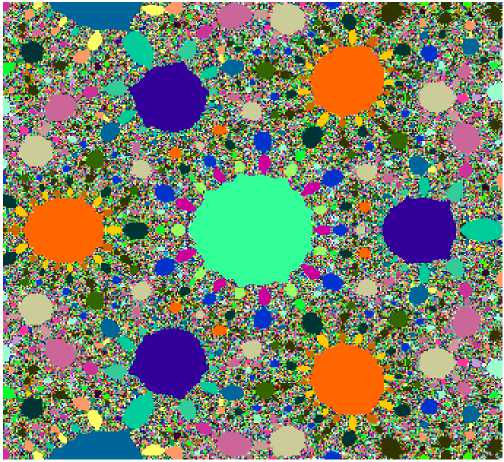
rings. We can
M
a
,
n
(
z
)
=
1
deduce that the rational map an 1 where a =--has no Herman zn+1 an rings. The Julia set of Ma n (z) is shown in Fig.2.
III. WAVELETS BASED ITERATED FUNCTIONS
Wavelets find applications and have significant impact in various scientific areas including geophysics, hydrodynamics, econometrics, data processing, image compression, detection of discontinuities, neural networks, etc [15]. One of the reasons wavelets have found so many uses and applications is that they are especially attractive from the computational point of view.
2
x
c
n
z
3
Computational efficiency of wavelets lies in the fact that wavelet coefficients in wavelet expansions for functions in Vq (resolution subspace in L2 (^d ) may be computed using matrix iteration, rather than by a direct computation of inner products: the latter would involve integration over Rd , and hence be computationally inefficient, if feasible at all. The deeper reason for why we can compute wavelet coefficients using matrix iteration is an important connection to the subband filtering method from signal/image processing involving digital filters, down-sampling and up-sampling. In this setting filters may be realized as functions m on a d-torus, e.g., quadrature mirror filters [16]. It would be interesting to adapt and modify the Haar wavelet, and the other wavelet algorithms to the Julia sets [17].
One of the applications of these IFSs, and their spectral theory, is to image processing [18] and [19]. IFSs include dynamical systems defined from a finite set of affine and contractive mappings in
R
d
, or from the branches of inverses of complex polynomials, or of rational mappings in the complex plane. A unifying approach to wavelets, dynamical systems, iterated function systems, self-similarity and fractals may be based on the systematic use of operator analysis and representation theory [20].
In terms of signal processing, what the two have in common, wavelets and IFSs, is that large scale data may be compressed into a few functions or parameters. In the case of IFSs, only a few matrix entries are needed, and a finite set of vectors in
R
d
must be prescribed. As is shown in [18], this can be turned into effective codes for large images. Similarly (see [21]) discrete wavelet algorithms can be applied to digital images and to data mining. The efficiency in these applications lies in the same fact: The wavelets may be represented and determined by a small set of parameters; a choice of scaling matrix and of masking coefficients, i.e., the coefficients
a
in the scaling identity Eqn. (3.1) below [22]. The scaling function
ф
satisfies an important equation, called the scaling equation. This is obtained by considering the function
ф
(
A
1
)
which lies in
V_
c
Vo
. Since the translates of
ф
form a basis for
V
, the scaling function is obtained:
1
-
1
. ф
(
A x
)
= 2
a^ф
(
x
-
k
)
,
(
x
e
Rd
)
ke Zd where (a^, ) ^ is a sequence of complex numbers. (3.1) Definition 3.1
Let
z
^
R
(
z
)
be a given polynomial. Let P be a finite set of distinct polynomials each of degree less than the degree of R. Let
K
2
(
R
,
P
)
be a space of functions F in
H
2
(
J
(
R
))
. We say that F is in
K
2
(
R
,
P
)
if there are functions
Fp
(
z
)
in
H
2
(
J
(
R
))
indexed by P such that
F
(
z
)
= 2
p
(
z Fp
(
R
(
z
))
p
e
P '
(3
.
2)
It is easy to see that each K2 (R, P) is a closed subspace in H2 (J(R)), so in particular it is a Hilbert space. The finite family P that enters Eqn.(3.2) is a family of generalized filters. It depends on the particular polynomial z ^ R(z) , and we can expect to find solutions to Eqn. (3.2) in Definition 3.1 from the kind of representations of the Cuntz algebras the authors studied in their work on wavelets on fractals [19]. In this paper we will deal with the complex iteration systems which generate Julia sets in the Riemann sphere.
IV. SIMULATION WITH SPTOOL
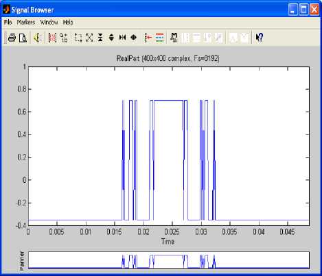
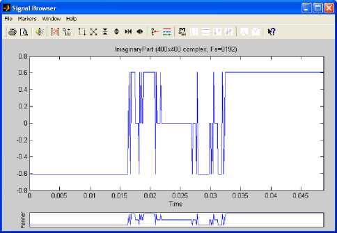
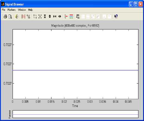
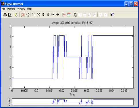
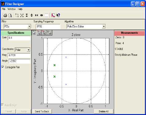
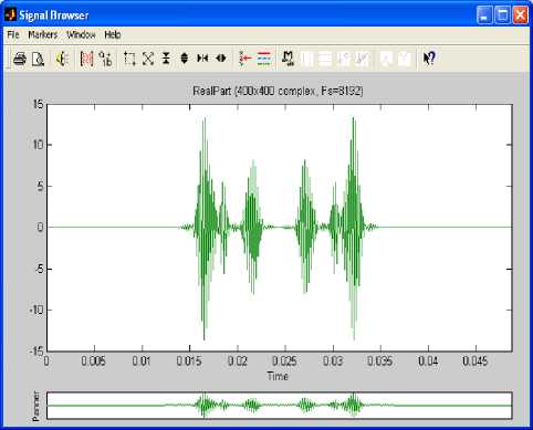
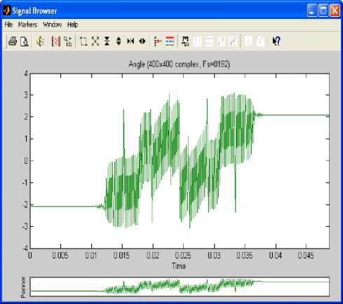
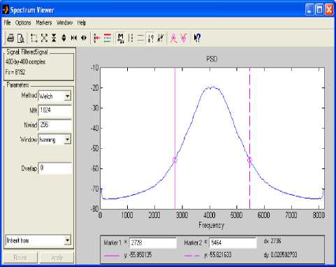
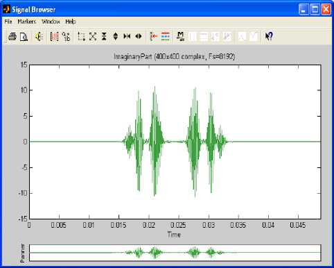
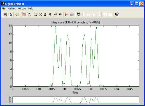
In this section we are interested in complex signals generated by importing the Julia set shown in Fig.1, from Matlab workspace to matlab signal processing tool with the sampling frequency of 8192Hz. This tool has three main components: signal section view, filter section view and edit as well as spectra section. These are used to visualize waveforms and spectra of several signals and make a qualified filter design. In order to use a complex signal under these processes the Julia fractal was imported as an array of 400 column index vectors, each of them having the real part, imaginary part, magnitude and phase angle. Fig.3, Fig.4, Fig.5 and Fig.6 show the sampled real part, imaginary part, magnitude and phase angle of the column index vector 1 respectively.
Let X(t) = [Xj (t) x2 (t) . . . Xm (t)] be the sampling vector signal Let r(t) = [r1(t) r2(t) . . . rm (t)] be the sampled vector signal Let У(t) = [Уi(t) У2(t) . . . Ут (t)] be the response of the band pass filter
Let
f
(
t
)
be the impulse response of the band pass filter
^ (
t
)
=
J
11
X
1
(
t
)
+
J
21
X
2(
t
)
+
...
+
J
m
,
X
,
(
t
)
=
^
J„Xt
(
t
) ;
i
=
k
=
1
I r1( t) = ZJ1 xk (t )| r2 (t) = J12X 1(t) + J22x2(t) + ... + Jm2Xm (t) = £ J^Xt (t) ;
=
k
=
1
I
r
2
(
t
)| =
J
E
Ji
2
Xk
(
t
)|
.
r
m
(
t
)
=
J
1
mX
1
(
t
)
+
J
2
mX
2
(
t
)
+
...
+
JmmXm
(
t
)
=
£
J™Xk
(
t^
i=k
=
1
I
r
m
(
t
)l
=
E
JmXk
(
t
)|
Since
r
(
t
)
=
X
(
t
)
X
J
is a complex signal, then, the magnitude of the sampled signal is given by:
I
r
(
t
)
=
7
r
12
(
t
)
+
r
22
(
t
)
+
...
+
r
m
2(
t
)
mm
Z
|
Z
J
j
X
k
(
t
)
j
=1
\
i
=
k
=1
Let
J
=
J
11
J
21
J
12
J
22
J
1
m
J
2
m
be
m
X
m
data
J
m
1
J
m
2
J mm
matrix representing the Julia set
J
(
f
)
in Fig.1. This data matrix is a complex matrix,
J
G
Z
m
X
m
, associated with
m
X
m
Pixels of the Julia set. In our case we have considered
m
=
400
in the Matlab programme that has generated the Julia set. The Matlab signal processing tool shows that the sampled vector signal generated out of the Julia set
J
(
f
)
is a complex signal with real part, imaginary part, magnitude and phase. In this section we attempt to express the sampled vector signal
r
(
t
)
in terms of sampling vector signal
x
(
t
)
as well as data matrix
J
representing the Julia set.
Fig.3. Real Part for Column Index Vector 1
In vector form
r
(
t
)
=
X
(
t
)
X
J
can be written as:
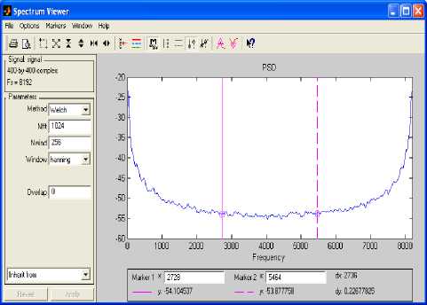
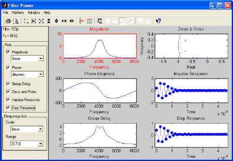
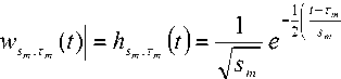
Fig.4. Imaginary Part for Column Index Vector 1 Fig.5. Magnitude for Column Index Vector 1 Fig.6. Angle for Column Index Vector 1 The power spectral density (PSD) of the sampled complex signal is shown in Fig.7. A stable band pass filter has been designed to analyze the complex signal in the sampling frequency range. Fig.8 shows magnitude, phase response, step response, group phase delay and other properties whereas Fig.9 indicates the pole–zero plot of the filter. The filtered real part, imaginary part, magnitude and phase angle of the column index vector 1 are shown in Fig.10, Fig.11, Fig.12 and Fig.13 show respectively. The filtering process has eliminated noise successfully. The power spectral density (PSD) of the filtered complex signal is shown in Fig.14. By definition the response of the band pass filter is given by the convolution of the impulse response f (t) of the band pass filter with the sampled vector signal r(t) = [r (t) r (t) . . . rm (t)]. Hence we get У (t) = f(t) * r (t) = J r (t)f(t - ^) d^ • Fig.8. Band Pass Filter Characteristics Fig.9. Band Pass Filter Pole-Zero Plot Apply the definition to each column, we get:
У
2
(
t )
=
r
2
(
t)
*
f
(
t)
=
J
r
2
(
t)f
(
t
-
°
) d
°
=
J
I
]Ё
J
,
2
X
k
(
t
)
I
f
(
t
-
CT
)
d
°
V,=k=1
=
L
j
2
J
x
k
(
t
)
f
(
t
-
°
)
d
°
=
k
=
1
У
1
(
t
)
=
r
i
(
t
)
*
f
(
t
)
=
J
r
i
(
t
)
f
(
t
-
°
)
d
°
( mk1
=
J L
J
,
i
x
k
(
t
)
f
(
t
-
°
)
d
°
V,= k=1
=
L
J
,
1
J
X
k
(
t
)
f
(
t
—
°
)
d
°
=
k
=
1
m ч 1 ,t (t) = L J, 1J xk(t)f(t- °) d° ,=k=1
=
cos
to
o
(
t
-
"
1
+
j
sin
to
o
(
t
-
"
1
1
h
,.
"
1
(
t
)
V
s
1
J
V
s
1
J.
w
s
2 ,
T
(
t
)
=
L
J
,
2
J
x
k
(
t
)
f
(
t
-
°
)
d
°
,
=
k
=1
cos
^
(
'
V
T
2
s
+
j
sin <
»0
(
t
V
-
T
2
s
2
hs t (t)
s
2
,
T
2 7
У
т
(
t
)
=
r
m
(
t
)
*
f
(
t
)
=
J
r
m
(
t
)
f
(
t
-
°
)
d
°
( m-, A
V
i
=
k
=
1
J
m
=
L
Jm
J
xk
(
t
).
f
(
t
—
°
)
d
°
=
k
=
1
y, (t)=ws, ,r, (t) = L J J xk (t) f (t-°) d° i=k=1 m
=
L
J
J
x
k
(
t
)
f
(
t
-
°
)
d
°
=
k
=
1
11 - t 1 11 - t cos tool------ | + j sin I I l V 3j J V 3j sj,Tjv 7 where (t T ? j m wmT ,Tm (t) = L Jm J xk (t)f (t- °)d° ,=k=1 cos <»0 (t — V sm t 1 — I + j sin too (t — Tm V sm ^ t (t) sm ,T m x ' The magnitude of the complex wavelet generated out of the Julia set of m x m Pixels, is given by: | Ч.Д t )| = hS1,T1(t ) = I ws 2,T 2 — e s1 — (t)| = hs2,T2 (t)= I--- e s2 (t — T1A2 s V 1 J (t — T"2 V s2 The phase of the complex wavelet generated out of the Julia set of m x m Pixels, is given by: hsj ,Tj(t )= -re e sj V s j J Ф5,T =^s 1,T1(t) Ф5 2,T2(t ) . . . Ф5- ,Tm(t The complex wavelet generated out of the Julia set of m x m Pixels, is given by: Ч г = 1ч г (t) Ч г (t) . . . Ч г (t) ] s,T L s 1,T1 v 7 s2,T2 v 7 sm ,Tm v 7 J Ф$1,тЛ t) = s1 Ф8г,T (t) =------2 2, 2 s2 t — T фsm ,"m(t) = — We can repeat the same steps on the rational map shown in Fig.2. Fig.10. Filtered Real Part for Column Index Vector 1 Fig.13. Filtered Angle for Column Index Vector 1 Fig.14. PSD of Filtered Julia Set П 2 х tan — Ma,2( z) = 1--Г3 z Fig.11. Filtered Imaginary Part for Column Index Vector 1 Fig.12. Filtered Magnitude for Column Index Vector 1 V. CONCLUSION This research aimed at the generation of wavelets in the dynamics of rational maps having Zhukovskii function. But the reasoning applied on these rational maps can be extended to any other rational map. Indeed we have compute Julia sets of the rational maps with 400 х 400 pixels for 500 iterations using Matlab programme. We have then imported the data associated with the Julia set from Matlab workspace to Signal Processing Tool and generated complex signals through the sampling process of 8192 Hz. The filtering process of these complex signals has eliminated noise successfully.The effect of the filter has generated wavelets on both real part and imaginary part of the complex signals generated by the Julia set. We have also found that the filtered complex signals have dominating frequency at half of the sampling frequency.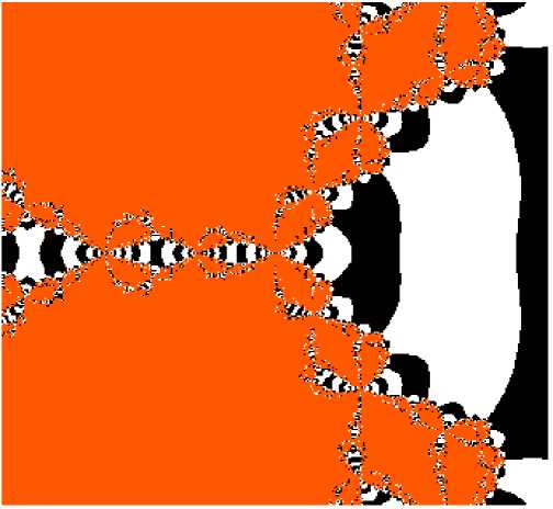
" r1( t)"
’ J11
J21 .
. . Jm 1 "
" X1( t) "
r2( t ) .
=
J12
.
.
J22 .
..
..
. . Jm2
.. .
.. .
X
X 2( t ) .
.
L rm (t )J
.
L J1 m
..
J2m .
.. .
. . Jmm J
.
LXm (t)J
rT(t) = JT X XT(t) = (X(t) X J)T
References Wavelet Based Some Julia Sets of Rational Maps Having Zhukovskii Function
- Jean-Bosco Mugiraneza, On Computing Some Julia Sets of Rational Maps Having Zhukovskii Function, Canadian Journal on Computing in Mathematics, Natural Sciences, Engineering and Medicine, Vol. 2 No. 7, pp: 187-202, August 2011, ISSN: 1923-1660, AM Publishers Corporation, Canada
- Dynamics of Rational Functions, Graduate Lecture Course, University of Bristol, Spring 2007
- Curtis T. McMullen, Frontiers in Complex Dynamics, University of California, Berkeley CA 94720, 16 February, 1994
- Alan F. Beardon, Iteration of Rational Functions: Complex Analytic Dynamical Systems. Number 132 in Graduate Texts in Mathematics. Springer-Verlag, New York, 1991.
- R. Bamón and J. Bobenrieth, The Rational Maps Have no Herman Rings, Proceedings of the American Mathematical Society, Volume 127, Number 2, February 1999, Pages 633-636 S 0002-9939(99)04566-9
- Robert L. Devaney, Dynamics of , Why the Case is Crazy, Boston University, February 2011
- D.J. Acheson, Elementary Fluid Dynamics, Clarendon Press, Oxford, UK, 1990
- Rachel W. Hall and Krešimir Josić, Planetary Motion and the Duality of Force Laws, SIAM, Vol. 42, No.1, pp.115-124, AMS:70F05,30A99,30C99, 2000
- Robert L. Devaney, Matt Holzer, and David Uminsky, Blow Up Points and Baby Mandelbrot Sets for Singularly Perturbed Rational Maps, 1991, Mathematical Subject Classification. Primary 37F45; Secondary 37F10.
- Jonathan Fraser, An Introduction to Julia Sets, April 16, 2009
- J. Milnor, Geometry and Dynamics of Quadratic Rational Maps, Experimental Mathematics (1) 2 (1993), 37 - 83. MR 96b:58094
- M. Lyubich, The dynamics of Rational Transforms: The Topological Picture, Russian Math. Surveys (4) 41 (1986), 3595. MR 88g: 58094
- M. Shishikura, On the Quasiconformal Surgery of Rational Functions, Ann. Sci. Ec. Norm.Sup. 20 (1987), 1 - 29. MR 88i:58099
- J. Milnor, Dynamics in One Complex Variable, 3rd Edition, Princeton University Press, 2006
- Shahriar Yousefi, Ilona Weinreich and Dominik Reinarz, Wavelet-Based Prediction of Oil Prices, Chaos Solitons and Fractals, Elsevier, November 2004
- Dorin Ervin Dutkay and Palle E.T. Jorgensen, Iterated Function Systems, Ruelle Operators, and Invariant Projective Measures, March 2008
- Palle E.T. Jorgensen and Myung-Sin Song, Comparison of Discrete and Continuous Wavelet Transforms, July 2007
- Michael Fielding Barnsley, Superfractals. Cambridge University Press, Cambridge, 2006.
- Dorin E. Dutkay and Palle E. T. Jorgensen, Wavelets on Fractals. Rev. Mat. Iberoamericana, 22(1):131–180, 2006.
- Myung-Sin Song, Analysis of Fractals, Image Compression and Entropy Encoding, Southern Illinois University Edwardsville, July 10, 2009
- Palle E. T. Jorgensen, Analysis and probability: Wavelets, Signals, Fractals, volume 234 of Graduate Texts in Mathematics, Springer, New York, 2006.
- Dorin Ervin Dutkay and Palle E.T. Jorgensen, Fourier Series On Fractals: A Parallel with Wavelet Theory, January 2008
