Wavelet Transform Techniques for Image Compression – An Evaluation

Memory and channel bandwidth are the prime constraints in image transmission and storage applications. In view of the growing energy requirements of wireless data services, the volume of multimedia data being transmitted over wireless channels may be reduced using various compression techniques, image compression entails transforming and organizing the data in an easy way of representation in which images of various types and sizes are compressed using different methodologies.

Image compression is one of the most visible applications of wavelet transforms additional to diversified fields as biomedical applications, wireless communications, computer graphics etc. [1]Wavelet based image coders like JPEG2000 standard easily outperform the traditional discrete cosine transform based JPEG image compression. Unlike in DCT based JPEG image compression, the performance of a wavelet based image coder depends to a large extent on the selected wavelet family but standard wavelets normally perform well with photographic images but most images do not possess similar statistical properties as photographic images like medical images, fingerprints, scanned documents and satellite images etc., Active research is carried out on multimedia data compression techniques like JPEG, JPEG2000 and MPEG with more emphasis on achieving high compression ratios, better peak signal to noise ratio (PSNR) and Less mean square error(MSE) measures without degrading the reconstructed image quality.

[2, 3] Wavelets provide good compression ratios for high resolution images and perform better than competing technologies like JPEG, in terms of signal to noise ratio and visual quality. Unlike JPEG, wavelets show no blocking affects but allows for a degradation of the image quality while preserving the significant details of the image. In JPEG2000 standard wavelet based image compression system the entire image is transformed and compressed as a single data object rather than block by block as in a DCT based compression system there by allowing uniform distribution of the compression error across the entire image to provide better image quality and high compression ratio.

This paper is organized as follows. Section 2 discusses the proposed transform based image compression system. Section 3 details the objective fidelity measures to assess the quality of reconstructed image. Section 4 briefs about discrete wavelet transform. Section 5 elaborates different wavelet families for image compression. Section 6 explains the results, followed by conclusion in section 7.

• II.    TRANSFORM BASED IMAGE COMPRESSION SYSTEM

Image compression techniques are broadly classified as lossy compression techniques and lossless compression techniques, depending on whether or not an exact replica of the original image could be constructed using the compressed image.

Lossless image compression techniques are limited in terms of compression ratios, they encode data exactly such that decoded image is identical to the original image. Lossless compression uses predictive encoding which uses the gray level of each pixel to predict the gray value of its right neighbor, the overall result is the reduction of redundancy in the data. Lossless image compression techniques are mainly preferred for applications with stringent requirements such as medical imaging and diagnosis etc.

[3, 12]Lossy compression techniques result in high compression ratios and are widely used based on the fact that decompressed image is only a close approximation to the original image.

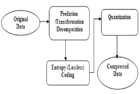
Figure 1. Lossy Image Compression Operation Sequence

Lossy image compression techniques normally involve Transform coding, Quantization and Entropy encoding operations. In transform coding every image is mathematically transformed similar to Fourier transform, separating image Information on gradual spatial variation of brightness, from regions with faster variations in brightness at edges of the image. Quantization is an irreversible operation in which the slowly changing information is transmitted entirely lossless while information that changes rapidly is transmitted with less accuracy. Transformation Coding techniques, Vector quantization, Fractal coding, Block Truncation coding and Sub band coding etc are few lossy compression techniques.

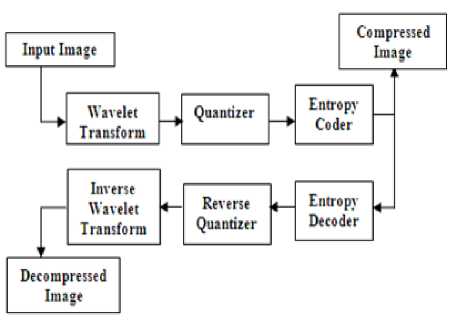
Figure 2. Transform based image compression system

Transform based compression techniques are the mostly used lossy compression techniques, as shown in Fig 2

Initially the input image is processed with selected wavelet Transform to decorrelate the input image; the transform coefficients so obtained are quantized to eliminate the psychovisual redundancy. A good quantizer normally assigns more bits for coefficients with more information content or perceptual significance and fewer bits for coefficients with less information content. The choice of a quantizer depends on the wavelet transform selected.

The last step in transform based quantization is entropy coding, which removes redundancy in the form of repeated bit patterns in the output of the quantizer. Here frequently occurring symbols are replaced with longer bit patterns, resulting in a small bit pattern. The most common entropy coding techniques are Run-Length Encoding (RLE), Huffman encoding, Arithmetic coding and Lempel-Ziv algorithms (LZW) .Arithmetic coder is more effective than others allowing arithmetic codes to outperform Huffman codes and consequently Arithmetic codes are more commonly used in wavelet based algorithms [3].

• III.    DESIGN METRICS

Digital image compression techniques are normally analyzed with objective fidelity measuring metrics like Peak Signal to Noise Ratio (PSNR), Mean Square Error (MSE), Compression Ratio (CR), Encoding time, Decoding time and Transforming time etc.[14]

• A.    Mean Square Error (MSE)

MSE refers to a sort of average or sum of squares of the error between two images. In analogy to standard deviation, taking the square root of MSE yields the root mean squared error or RMSE.

MSE for monochrome images is given by

NN

12∑∑[X(i, j)-Y(i, j)]2                               (1)

MSE for color images is given by

NN

∑∑{[r(i, j)-r*(i, j)]2+[g(i, j)-g*(i, j)]2

N ² i j                                                            (2)

+[b(i, j)-b*(i, j)]2}

Where r (i, j), g (i, j) and b (i, j) represents the color pixels at location (i, j) of the original image. r* (i, j), g* (i, j) and b*(i, j) represent the color pixel of the reconstructed image, while N x N denotes the size of the pixels of the color images[2].

• B.    Peak Signal to Noise Ratio (PSNR)

Peak signal to Noise Ratio is the ratio between signal variance and reconstruction error variance. PSNR is usually expressed in Decibel scale. The PSNR is mostly used as a common measure of the quality of reconstruction in image compression etc.

PSNR = 10log                                (3)

• 10 MSE

Here 255 represent the maximum pixel value of the image, when the pixels are represented using 8 bits per sample. PSNR values range between infinity for identical images, to 0 for images that have no commonality. PSNR is inversely proportional to MSE and CR as well i.e PSNR decreases as the compression ratio increases, for an image.

• C.    Compression Ratio (CR)

Compression ratio is defined as the ratio between the original image size and compressed image size.

Origianal Im age Size

Compression Ratio =

Compressed Im age Size

• IV.    WAVELET TRANSFORMS

[5]Mathematical transforms are used to translate the information of signals into different representations. For example the Fourier transforms converts the signal between time and frequency domains, but Fourier transform failed to provide information related to particular frequencies at specific times. This problem is solved with window based Short Term Fourier Transform (STFT) technique in which different parts of a signal can be viewed. However Heisenberg’s Uncertainty Principle states that as the resolution of the signal is improved in time domain by Zooming on different sections, the resolution gets worse in frequency domain. Hence a method of multiresolution is needed that can allow certain parts of the signal to be resolved in time and remaining parts in frequency domain.

The power of wavelets comes from the use of multiresloution rather than examining entire signals through the same window, different parts of the wave are viewed through different sized windows where high frequency parts of the signal uses small window to give good time resolution while the low frequency parts uses big window to extract good frequency information.

[3]Wavelet transform analysis represents image as a sum of wavelet functions with different locations and scales. Wavelet transforms exhibit high décorrelation and energy compaction properties. Problems like blocking artifacts and mosquito noise are absent in wavelet based image coders, also distortion due to aliasing is totally eliminated through design of proper filters. These properties made wavelets suitable for image compression. Similar to other linear transforms, wavelet transforms reduce the entropy of an image i.e. the wavelet coefficient matrix has lower entropy than the image itself and hence coefficient matrix is more efficiently encoded.

Wavelet transform allows good localization in frequency and space, there exist fast O (n Log n) algorithms for implementation. Wavelet decomposition of an image involve a pair of waveforms to represent the high frequencies Corresponding to the detailed parts of an image (wavelet function) clearly showing the Vertical, Horizontal and Diagonal details of the image while the low frequencies or Smooth parts of an image (scaling function) correspond to approximation coefficients. If the high frequency coefficients are very small they can be set to zero without significantly changing the image , the value below which these details can be considered small enough to be set to zero is known as threshold. The greater the number of zeros the greater is the compression that can be achieved.

• [1]    The amount of information retained by an image after encoding and decoding operations is known as energy retained, which is proportional to the sum of squares of pixel values. If the energy retained is 100% then the compression is lossless as the image can be reconstructed exactly. This occurs when the threshold value is set to zero; it means that the details have not been changed. If any values are changed then energy is lost leading to a lossy compression. Ideally, during compression the number of zeros and the energy retention are as high as possible. However, as more zeros are obtained more energy is lost; hence a balance among the two is required.

Wavelet transforms are classified to be continuous and discrete. For long signals continuous wavelet transform is time consuming, as it needs to be integrated at all times. Discrete wavelet transform (DWT) can be implemented through sub band coding and is useful because it can localize signals in time and scale, whereas the DFT or DCT can localize signals in the frequency domain. DWT is obtained by filtering the signal through a series of digital filters of different scales. The scaling operation is done by changing the resolution of the signal through sampling [13].

• V. WAVELET FAMILIES

Different families of wavelet functions are developed for DWT that are compactly supported, orthogonal and biorthogonal and are characterized by the low-pass and high-pass analysis filters and synthesis filters. Haar, Daubechies, Symlets, Coiflets, Meyer, Mexicanhat and Morlet etc are few families of wavelets available [12].

The Haar, Daubechies, Symlets and Coiflets are supported by orthogonal wavelets while the Meyer, Mexicanhat; Morlet wavelets are symmetric in shape. Based on the scaling function and ability to analyze the signal, wavelets are chosen for any particular application [14].Haar, Daubechies, Symlets, Coiflets and biorthogonal wavelets are few DWT families discussed in this work.

• A. Haar Wavelets

  The Haar matrix proposed in 1909 by Alfred Haar is the simplest possible wavelet and is a very fast transform. The basis vectors of the Haar matrix are sequentially ordered. In mathematics, the Haar wavelet is a sequence of rescaled “square-shaped” functions. Technical disadvantage of Haar wavelet is that it is not continuous and therefore not differentiable and resembles a step function. This property is an advantage for analyzing signals with sudden transitions, like monitoring of tool failures in machines. It represents same wavelet as Daubechies 1.

3 =

з + уз

(4.3)

4 =

1 + Уз

(4.4)

[5, 9]Daubechies wavelet transforms are defined in the same way as the Haar wavelet by computing running averages and differences through scalar products with scaling signals and wavelets. For high order Daubechies wavelets DbN, N denotes the order of wavelet and the number of vanishing moments, Daubechies wavelets have highest number(A) of vanishing moments for given support width N=2A,The length of the wavelet transform is easy to put into practice using the fast wavelet transform, the approximation and detail coefficients are of length

/ n - 1 \

Floor (        ) + N

If n is the length of f (t), this wavelet has balanced frequency responses but non-linear phase responses.

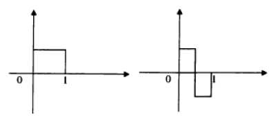
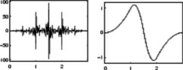
Figure 3. Scaling and Wavelet functions of HAAR

Haar Transform has poor energy Compaction for images and is real and orthogonal i.e. Hr = Hr*, the basis vectors of Haar matrix are always sequence ordered [11].

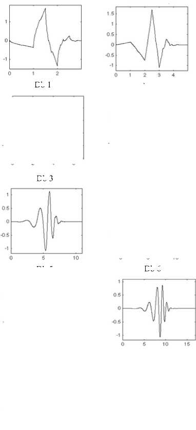
B. Daubechies Wavelets

A major problem in the development of wavelets during the 1980’s was the search for scaling functions that are compactly supported, orthogonal and continuous. These scaling functions were first constructed by Ingrid Daubechies, this construction amounts to finding the low pass filter h, or equivalently, the Fourier series. Ingrid Daubechies invented compactly supported orthonormal wavelets- thus making discrete wavelet analysis practicable [7]. Daubechies wavelet transform signal is defined by the scaling and wavelet functions that are expressed in terms of and β coefficients, respectively.

1 =

1 + Уз

(4.1)

(4.2)

Db 3

Db 8

Db 1

Db 6

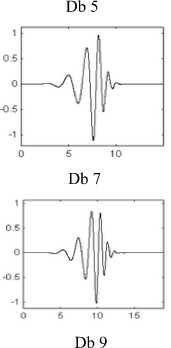
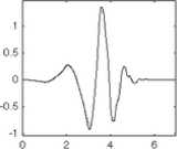
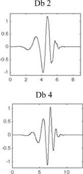
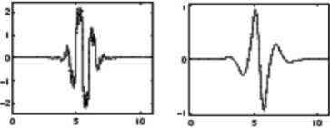
Figure 4. Wavelet Functions of Daubechies

Wavelets with fewer vanishing moments give less smoothing and remove less details, but wavelets with more vanishing moments produce distortions. Daubechies wavelets are widely used to solve broad range of problems like for example, self-similarity Properties of a signal or fractal problems, signal discontinuities etc. The wavelet functions Psi of the next nine members of the family are listed in fig.4, in which x-axis represents the time and y-axis represents the frequency.

• C.    Symlet Wavelets

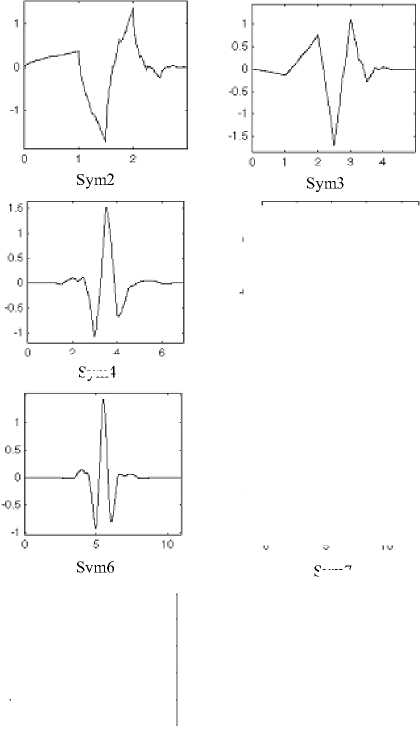
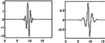
The scaling/Wavelet functions of Daubechies wavelets are far from symmetry because Daubechies wavelets select the minimum phase square root such that the energy concentrates near the starting point of their support, while Symlets select each other set of roots to have closer symmetry with linear complex phase. Symlets are nearly symmetrical wavelets Proposed by Daubechies as modifications to the Db family, apart from the symmetry, remaining other properties of Daubechies and Symlet families are similar [4,8].

Symlets, as shown in fig.5, when applied to signal performs better and the Signal to Noise Ratio (SNR) of reconstructed or denoised signal is improved. Symlets are found to be more efficient in denoising applications.

Sym4

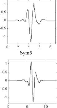
Sym7

Sym8

Figure 5. Wavelet functions of Symlets

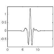
• D.    Coiflet Wavelts

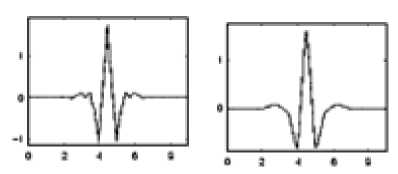
Coiflets and the well known Daubechies wavelets are similar in a certain level, but the Coiflet was constructed with vanishing moments not only for wavelet function φ(x), but also for scaling function ø(x). .Coiflets, as shown in fig.6, are near symmetric; their wavelet functions have N/3 vanishing moments and scaling functions N/3 – 1. They are used in many applications using Calderon-Sigmund Operators. Both scaling and Wavelet functions have to be normalized by a factor 1/^г 2 .The scaling function of coiflets exhibit interpolating characteristics, which implies that this wavelet allows a good approximation of polynomial function at different resolutions.[7] Further, the property of symmetry in coiflets is desirable in signal analysis work due to the linear phase of the transfer function, although coiflet method is less flexible in visualizing any frequency of interest, its discrete form is useful for digital implementation.

Coif 5

Figure 6. Wavelet functions of Coiflets

The wavelet function has 2N moments equal to 0 and the scaling function has 2N – 1 moments equal to 0. The wavelet function and the scaling functions have a support of length 6N-1. Coiflet wavelet basis function is embedded within the wavelet transform scheme. This wavelet can be derived from a multi resolution analysis such that the scaling function has a certain number of vanishing moments. Some useful features are

• i)    This method allows good approximation of polynomial functions at different resolutions, thereby increasing the computation efficiency of the analysis.

• ii)    As with other wavelet transforms, Coiflet transform can present both frequency and time information in an integral scheme. Visualization of signal characteristics can be easily achieved.

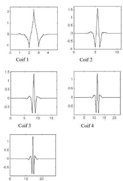
• E.    Biorthogonal Wavelets

Biorthogonal wavelets extend the family of orthogonal wavelets and have applications in signal and image processing. The periodic biorthogonal wavelet transforms are realized by Matrix-vector products with sparse, structured matrices [7, 9]. An open fact in filter theory community is that when same FIR filters are used for decomposition and reconstruction process, the symmetry and Perfect reconstructions are totally incompatible. To circumvent this difficulty, dual scaling and wavelet functions with following properties are used:

• i)    They are zero outside a segment and Calculation algorithms maintained are simple.

• ii)    Filters associated are symmetrical.

• iii)    Functions used for calculations are easier to build than those used in Daubechies wavelets.

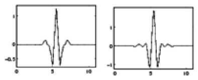
Biothogonal wavelets, as shown in figs.7 to 8, exhibit the property of linear phase for signal and image reconstruction, by using two wavelets for decomposition and reconstruction.The asymmetric nature of Biorthogonal wavelets causes artifacts at the borders of wavelet subbands. These wavelets along with Meyer wavelets are capable of perfect reconstruction.

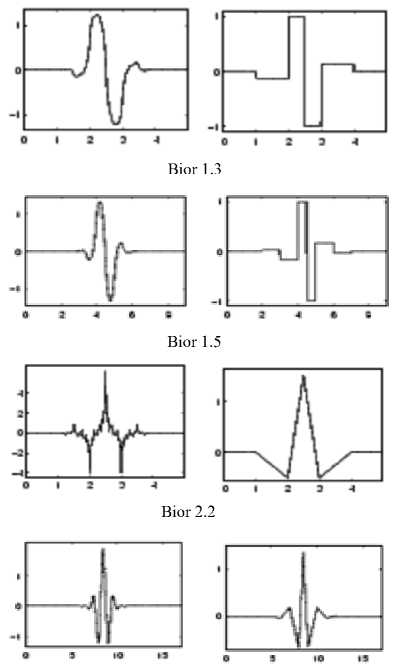
Bior 2.8

Figure 7. Biorthogonal Wavelet Families

Bior 3.1

Bior 3.5

Bior 3.9

Bior 4.4

Bior 5.5

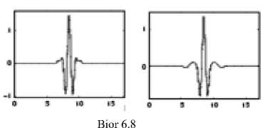
Figure 8. Biorthogonal Wavelet Families

• VI.    EXPERIMENTAL ANALYSIS

In the proposed analysis work, different gray scale images and color images with varying content of details are considered for two level decomposition as well as reconstruction using different hand designed wavelets families like Haar, Daubechies, Symlets, Coiflets and Biorthogonal wavelets. Selected bench mark image is decomposed with desired wavelet transform; Metrics PSNR, CR and MSE so obtained are tabulated for analysis after simulation in matlab environment.

Image 1: High Detailed Image

Figures.9 to 13 and Table.1 of High detailed image clearly imply that, of all daubechies wavelets, Db2 produced high value of PSNR while the Compression ratio is more for Db4 family, Coif1 and Coif2 produced better values of PSNR and CR In case of symlets, SYM4 and SYM6 wavelets have better PSNR and CR values. Bior4.4 and Bior3.3 generated large values of PSNR and CR.

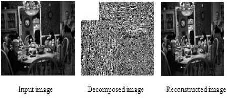
Figure 9. Daubechies Images

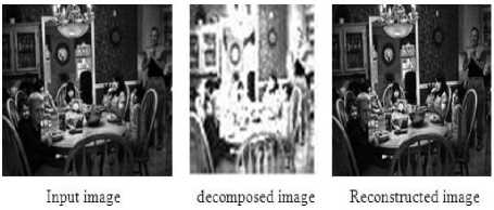
Figure 10. Coiflet Images

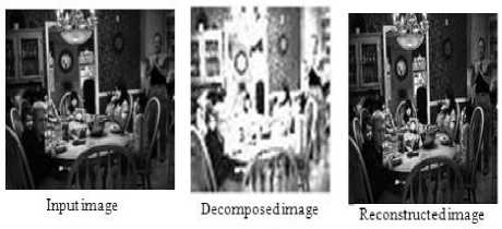
Figure 11. Symlet Images

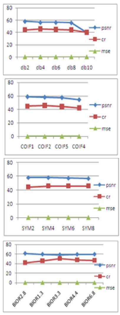
TABLE 1. PERFORMANCE COMPARISON BETWEEN DIFFERENT WAVELETS ON HIGH DETAIL IMAGE

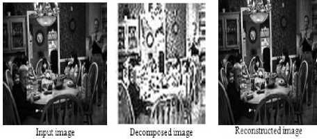
Figure 12. Biorthogonal Images

TABLE 1.1

256x256 Image	PSNR	CR	MSE
Db2	44.1807	44.5202	2.4832
Db4	43.5687	45.7569	2.8590
Db6	44.0453	44.9358	2.5619
Db8	43.8065	43.9987	2.7067
Db10	43.6212	40.3217	2.8246

Input image

Re c onstructe d image

Decomposed image

Figure 16. Symlet Images

TABLE 1.2

256x256 Image	PSNR	CR	MSE
Coif1	44.2141	44.7390	2.4641
Coif2	43.8441	45.8396	2.6833
Coif4	43.6987	42.1627	2.7747
Coif5	43.6856	42.4035	2.7830

TABLE 1.3

256x256 Image	PSNR	CR	MSE
Sym2	44.1807	44.5203	2.4832
Sym4	44.2005	45.6619	2.4719
Sym6	43.9502	45.7475	2.6185
Sym8	43.9125	45.6508	2.6414

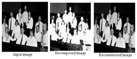
Figure 17. Biorthogonal Images

TABLE 1.4

256x256 Image	PSNR	CR	MSE
Bior1.3	43.7118	42.0138	2.7663
Bior2.8	41.3308	45.5531	4.7863
Bior3.3	40.0025	50.9124	6.4987
Bior4.4	44.4878	47.5693	2.3137
Bior6.8	44.1946	47.2618	2.4753

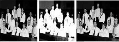
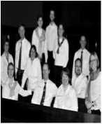
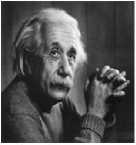
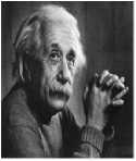
Image 2: Staff group image

Figures.14 to 18 and Table.2 of staff group image imply that, Db4 and Db2 wavelets produced high values of PSNR and CR value, on the other hand Coif2 and Coif1 wavelets resulted in better values of PSNR and CR, Sym4 wavelet generated better PSNR and CR values as well. While Bior4.4 wavelet produced better values of PSNR and CR of all biorthogonal family wavelets in contrast Bior4.4 wavelet produced the least value of CR.

Input image

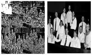
2-level decomposition Re constructed image

Figure 14. Daubechies Images

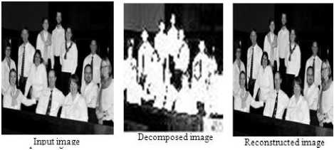
Figure 15. Coiflet Images

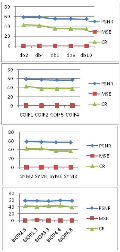
TABLE 2. PERFORMANCE COMPARISON BETWEEN DIFFERENT WAVELETS ON STAFF GROUP IMAGE

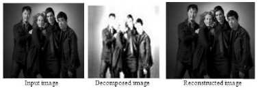
Figure 20. Coiflet Images

TABLE 2.1

256x256 Image	PSNR	CR	MSE
Db2	43.9405	42.8586	2.6244
Db4	45.9219	42.2732	1.6630
Db6	43.3411	36.0295	3.0128
Db8	43.9733	35.3813	2.6047
Db10	44.6924	34.7575	2.2072

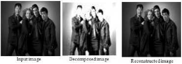
Figure 21. Symlet Images

TABLE 2.2

256x256 Image	PSNR	CR	MSE
Coif1	44.9805	43.0931	2.0655
Coif2	45.0981	37.5502	2.0104
Coif4	44.8458	37.4942	2.1306
Coif5	45.1981	37.4678	1.9646

TABLE 2.3

256x256 Image	PSNR	CR	MSE
Sym2	43.9405	42.6586	2.6244
Sym4	45.4329	43.1069	1.8612
Sym6	44.2020	37.1290	2.4711
Sym8	43.1248	37.1578	3.1667

TABLE 2.4

256x256 Image	PSNR	CR	MSE
Bior1.3	42.6002	42.5236	3.5733
Bior2.8	44.0403	41.1278	2.5648
Bior3.3	41.4665	43.1385	4.6391
Bior4.4	45.4631	44.5709	1.8483
Bior6.8	42.7644	38.6246	3.4407

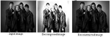
Figure 22. Biorthogonal Images

Image 3: Medium Detailed Image1

Figures.19 to 23 and Table.3 of medium detailed image clearly imply that, Db8 and Db4 wavelets have better values of PSNR and CR of the order 48.6538 and 61.2029, while the COIF5 wavelet produced large values of PSNR and CR. In the case of symlets it was observed that SYM6 family generated large values of PSNR and CR, However, Bior4.4 and Bior2.8 wavelets produced large values of PSNR and CR.

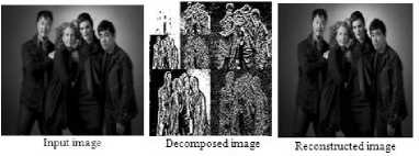
Figure 19. Daubechies Images

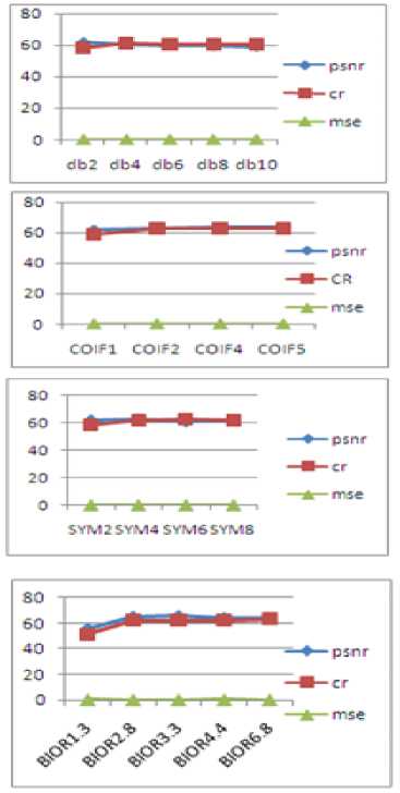
TABLE 3. PERFORMANCE COMPARISON BETWEEN

DIFFERENT WAVELETS ON MEDIUM DETAIL IMAGE1

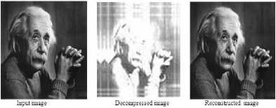
Figure 25. Coiflet Images

TABLE 3.1

256x256 Image	PSNR	CR	MSE
Db2	46.4657	58.5535	1.4673
Db4	46.9986	61.2029	1.2979
Db6	44.9210	60.4319	2.0940
Db8	48.6538	60.1944	0.8866
Db10	45.0492	60.1739	2.0331

TABLE 3.2

256x256 Image	PSNR	CR	MSE
Coif1	45.5252	58.9796	1.8221
Coif2	47.0560	62.9460	1.2808
Coif4	44.9459	62.7228	2.0820
Coif5	47.8653	63.0974	1.0630

TABLE 3.3

256x256 Image	PSNR	CR	MSE
Sym2	46.4657	58.5535	1.4673
Sym4	48.4667	61.6918	0.9256
Sym6	48.6160	62.7131	0.8943
Sym8	46.9712	61.8659	1.3060

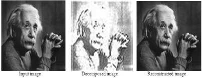
Figure 27. Biorthogonal Images

TABLE 3.4

256x256 Image	PSNR	CR	MSE
Bior1.3	47.3118	51.1779	1.2075
Bior2.8	42.9557	62.8143	3.3924
Bior3.3	45.6821	62.4839	1.7514
Bior4.4	47.9933	62.2816	1.0322
Bior6.8	47.5885	63.4034	1.1330

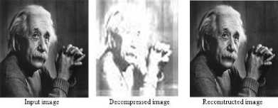
Figure 26. Symlet Images

Image 4: Medium Detailed Image2

Figures.24 to 28 and Table.4 of medium detailed image2 clearly imply that in the case of daubechies wavelets, Db6 wavelet produced better values of PSNR and CR, while Coif5 and Coif2 wavelets produced large values of PSNR and CR. In the case of symlets, Sym8 family produced better values of PSNR and CR as well, while Bior6.8 and Bior3.3 wavelets of biorthogonal family generated better values of PSNR and CR.

Input image

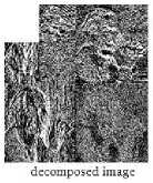
Figure 24. Daubechies Images

Reconstructed image

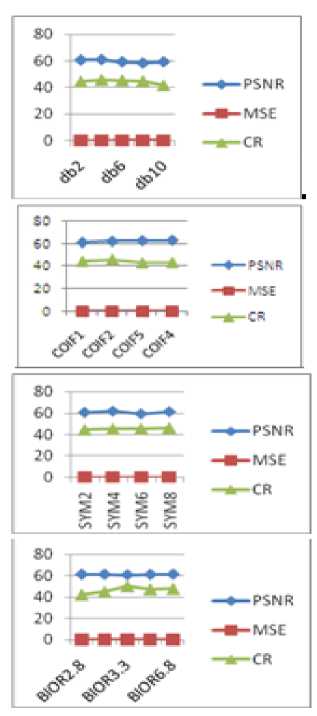
TABLE 4. PERFORMANCE COMPARISON BETWEEN

DIFFERENT WAVELETS ON MEDIUM DETAIL IMAGE2

Inputimage          De compose dimage        Reconstiuctedimage

Figure 30. Coiflet Images

TABLE 4.1

256x256 Image	PSNR	CR	MSE
Db2	44.9768	45.3677	2.0672
Db4	45.5209	46.7707	1.8238
Db6	45.7784	46.3030	1.7189
Db8	44.6593	45.8205	2.2241
Db10	44.4693	42.4157	2.3236

TABLE 4.2

256x256 Image	PSNR	CR	MSE
Coif1	45.2384	45.1643	1.9465
Coif2	45.0539	46.9520	2.0309
Coif4	45.3413	43.7697	1.9008
Coif5	46.0075	44.1976	1.6306

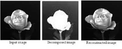
Figure 31. Symet Images

TABLE 4.3

256x256 Image	PSNR	CR	MSE
Sym2	44.9768	45.3677	2.0673
Sym4	45.5546	46.5212	1.8097
Sym6	44.8846	46.7163	2.1116
Sym8	45.9079	47.4649	1.6684

TABLE 4.4

256x256 Image	PSNR	CR	MSE
Bior1.3	44.0214	42.3772	2.5760
Bior2.8	43.6919	45.8234	2.7790
Bior3.3	40.9797	51.1180	5.1893
Bior4.4	45.8512	48.3373	1.6903
Bior6.8	45.5049	48.7441	1.8306

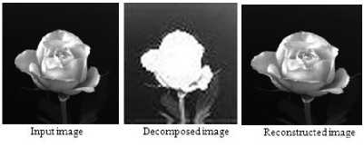
Figure 32. Biorthogonal Images

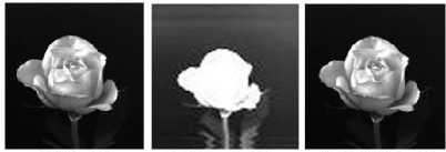
Image 5: Less Detailed Rose Image

Figures.29 to 33 and Table.5 of less detailed Rose image clearly imply that in the case of daubechies wavelets Db6 and Db2 wavelets produced better values of PSNR and CR of order 46.0933and 0.0691, COIF4 wavelet produced large PSNR value of 45.4990.In the case of symlets Sym4 wavelet family produced high value of PSNR of order 46.4155. While the Bior4.4 and Bior1.3 wavelets produced large values of PSNR and CR of order 46.6635 and 27.2914.

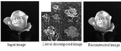
Figure 29. Daubechies Images

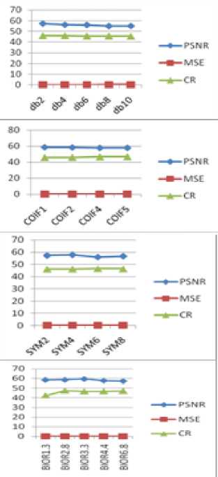
TABLE 5. PERFORMANCE COMPARISON BETWEEN DIFFERENT WAVELETS ON LESS DETAIL ROSE IMAGE

TABLE 5.1

256x256 Image	PSNR	CR	MSE
Db2	41.9606	0.0691	4.1402
Db4	43.4303	0.5123	2.9516
Db6	46.0933	0.2356	1.5986
Db8	42.0627	0.7834	4.0440
Db10	45.0702	0.3412	1.7622

TABLE 5.2

256x256 Image	PSNR	CR	MSE
Coif1	43.7609	0.6732	2.7352
Coif2	42.6858	0.2476	3.5035
Coif4	45.4990	0.2134	1.8331
Coif5	42.7457	0.3212	3.4555

TABLE 5.3

256x256 Image	PSNR	CR	MSE
Sym2	41.6906	0.0691	4.1402
Sym4	46.4155	0.4323	1.4843
Sym6	45.7680	0.3243	1.7226
Sym8	43.8461	0.2321	2.6819

TABLE 5.4

256x256 Image	PSNR	CR	MSE
Bior1.3	43.7508	27.2914	2.7415
Bior2.8	39.8109	0.3212	6.7919
Bior3.3	39.7653	0.2322	6.8036
Bior4.4	46.6635	06756	1.4019
Bior6.8	46.5071	0.4344	1.4534

Different color images have also been considered for analysis however the experimental results of two of them are tabulated but it was observed that the metrics so obtained for color images are numerically less in magnitude.

Image 6: Color Image 1

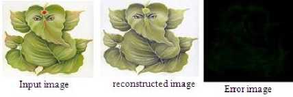
Figure 34. Daubechies Images

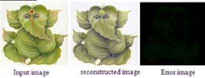
Figure 35. Coiflet Images

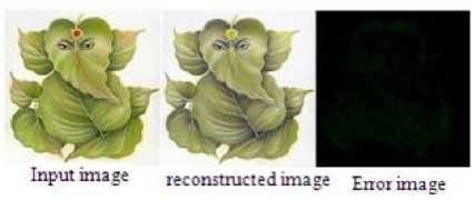
Figure 36. Symlet Images

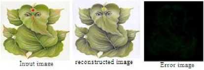
Figure 37. Biorthogonal Images

TABLE 6. PERFORMANCE COMPARISON BETWEEN

DIFFERENT WAVELETS OF COLOR IMAGE1

TABLE 6.1

256x256 Image	PSNR	CR	MSE
Db2	23.6354	49.0396	282.1884
Db4	24.9187	54.2091	209.5115
Db6	22.9369	56.1628	330.6647
Db8	23.1564	52.2848	314.3704
Db10	25.1855	52.8891	192.5421

TABLE 6.2

256x256 Image	PSNR	CR	MSE
Coif1	24.6266	49.8163	224.0912
Coif2	23.9378	56.7202	262.6008
Coif4	23.9871	56.0119	259.6391
Coif5	24.0328	52.9719	256.9158

TABLE 6.3

256x256 Image	PSNR	CR	MSE
Sym2	23.6254	49.0396	282.1884
Sym4	25.9718	54.3448	164.3993
Sym6	22.2935	57.1390	383.4689
Sym8	25.7423	58.6204	173.3189

TABLE 6.4

256x256 Image	PSNR	CR	MSE
Bior1.3	22.0834	42.9101	402.4793
Bior2.8	26.0250	52.7263	162.3979
Bior3.3	27.0686	55.2517	127.7095
Bior4.4	23.8721	53.5265	266.6091
Bior6.8	22.9935	56.0200	326.3816

TABLE 7.4

256x256 Image	PSNR	CR	MSE
Bior1.3	24.0607	43.8204	255.2753
Bior2.8	24.5585	47.8119	227.6307
Bior3.3	23.8916	49.8410	265.4142
Bior4.4	24.9968	47.0308	205.1804
Bior6.8	23.9385	46.7753	262.5622

Figures.34 to 37 and Table.6 of color image1 clearly imply that in case of daubechies wavelets, Db10 and Db6 wavelets have produced better values of PSNR and CR of order 25.2855 and 56.1628, while the Coif5 and Coif2 wavelets produced better values of PSNR and CR of order 24.0328 and 56.7202. In the case of symlets Sym8 wavelets produced better values of PSNR and CR of order 25.7423 and 58.0204 while the Bior3.3and Bior6.8 wavelets produced large values of PSNR and CR of order of 27.0686 and 56.0200.

Image 7: Color Image2

Figures.38 to 41 and Table.7 of color image2 clearly imply that in case of daubechies wavelets, Db4 and Db2 wavelets have produced better values of PSNR and CR, while the Coif1 and Coif2 wavelets produced better values of PSNR and CR. In the case of symlets Sym6 and Sym4 wavelets produced better values of PSNR and CR while the Bior4.4 and Bior3.3wavelets produced large values of PSNR and CR.

TABLE 7. PERFORMANCE COMPARISON BETWEEN DIFFERENT WAVELETS ON COLOR IMAGE2

TABLE 7. 1

256x256 Image	PSNR	CR	MSE
Db2	24.7468	45.1042	211.9217
Db4	23.4023	45.1350	297.0653
Db6	22.7566	44.3731	344.6845
Db8	22.8613	43.7797	336.4746
Db10	22.6365	43.5256	354.3553

TABLE 7.2

256x256 Image	PSNR	CR	MSE
Coif1	24.7242	45.2832	219.1102
Coif2	24.0395	45.6829	256.5255
Coif4	23.6890	45.5180	278.0878
Coif5	23.6474	40.4173	280.7782

TABLE 7.3

256x256 Image	PSNR	CR	MSE
Sym2	24.7468	45.1042	217.9717
Sym4	23.8829	45.5464	265.9417
Sym6	24.2779	45.4408	242.8263
Sym8	22.8482	45.5178	337.4881

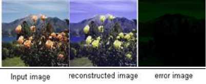
Figure 38. aubechies Images

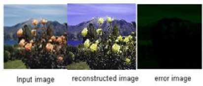
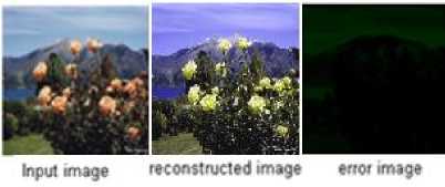
Figure 40. Symlet Images

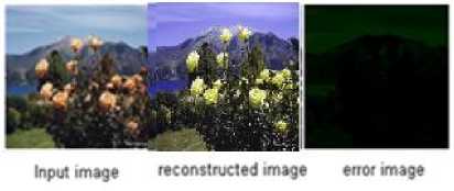
Figure 41. Biorthogonal Images

• VII.    CONCLUSION

This work is mainly focused upon the comparison and analysis of image compression metrics derived by the application of different wavelets like Haar, Daubechies, Coiflet, Symlet and Biorthogonal wavelets etc on various selected bench mark gray scale and color images of varying content and details. In total around 19 different wavelet transform functions are considered for the analysis. However the experimental results of 5 gray scale and 2 color images are presented here. The entire analysis involved round 126 encoding and decoding operations.

In the case of gray scale images it was observed that Daubechies family wavelet Db8 produced highest PSNR of order 48.6538 for Medium detail image1, while the Biorthogonal family wavelet Bior6.8 produced highest CR of order 63.4034 for the same Medium detail image1.

In the case of color images it was observed that Biorthogonal family wavelet Bior3.3 and Symlet family wavelet Sym6 produced better PSNR and CR values of order 27.0686 and 57.1390 for the same color image1-ganesh.

The results obtained clearly indicate that Biorthogonal functions offer good compression performance than remaining ones; however the Daubechies functions do perform better in statistical terms. Since each wavelet filter gives a different performance for different fidelity metrics and different images, it can be concluded that compression performance depends on the size and content of the image therefore it is appropriate to tailor the choice of wavelet based on image size and content for desired quality of reconstructed image.

• VIII.    ACKNOWLEDGEMENTS

The authors express their sincere thanks to the anonymous referees for their constructive comments and gratitude to the management of LIET for provision of excellent facilities. Thanks to the passed out graduate engineers for their contribution.