A Biometric System Based on Single-channel EEG Recording in One-second

Автор: Shaimaa Hagras, Reham R. Mostafa, Ahmed Abou Elfetouh

Журнал: International Journal of Intelligent Systems and Applications @ijisa

Статья в выпуске: 5 vol.12, 2020 года.

Бесплатный доступ

In recent years, there are great research interests in using the Electroencephalogram (EEG) signals in biometrics applications. The strength of EEG signals as a biometric comes from its major fraud prevention capability. However, EEG signals are so sensitive, and many factors affect its usage as a biometric; two of these factors are the number of channels, and the required time for acquiring the signal; these factors affect the convenience and practicality. This study proposes a novel approach for EEG-based biometrics that optimizes the channels of acquiring data to only one channel. And the time to only one second. The results are compared against five commonly used classifiers named: KNN, Random Forest (RF), Support Vector Machine (SVM), Decision Tables (DT), and Naïve Bayes (NB). We test the approach on the public Texas data repository. The results prove the constancy of the approach for the eight minutes. The best result of the eyes-closed scenario is Average True Positive Rate (TPR) 99.1% and 98.2% for the eyes-opened. And it reaches 100% for multiple subjects.

Еще

Biometrics, Electroencephalogram, Hjorth parameters, K-Nearest Neighbor, Naïve Bayes, Random Forest, and Support Vector Machine

Короткий адрес: https://sciup.org/15017512

IDR: 15017512 | DOI: 10.5815/ijisa.2020.05.03

Текст научной статьи A Biometric System Based on Single-channel EEG Recording in One-second

Published Online October 2020 in MECS

Using EEG as a biometric has been suggested in many studies [1], and it has achieved high accuracy results in most of them. EEG as a biometric has several advantages over the conventional biometrics in that EEG is more secure as it is impossible to be imitated or copied for fraud purposes. EEG signals, also, are highly affected by alcohol and drugs so the alcoholic and drug abusers will produce unacceptable signals, and thus, it will be useful in many systems that need a full concentration from the user such as driving, and military work. Moreover, EEG signals are highly affected by stress and mood that makes it difficult to force any person to produce the correct and acceptable signal. EEG signals are suitable for both static and continuous authentication (CA) systems. Furthermore, it can be used only by living subjects. On the other hand, there exist some constraints of the EEG-based biometrics applications, such as mindreading possibility, other constraints concerning the characteristics of the EEG signals; such as weakness, sensitivity and difficult to be trained.

The main stages of any EEG-based biometrics system are scenarios of capturing the signal, Feature extraction and classification. Scenarios: according to the published studies, many different scenarios of capturing EEG signals have been used in the literature: resting with EC, resting with EO, responding to stimuli [2, 3], performing a set of mental tasks (mental computations [4], imagined speech [5], and imagined movement [6]) where some mental tasks are more appropriate for EEG-based human recognition than others, and involve a particular movement such as moving a single finger [7]. The spatial distribution of the brain activations strongly dependent upon either the person’s mental state or the activity performed during the acquisition [8]. For each designed scenario there is an optimal electrode configuration based on the number of channels, their positions, and their density. The less time needed for the human test, the more positive user experience with the system is achieved [9]. Resting scenario provides the most user-friendly scenario as it does not request any instructions to the users only relax. Moreover, it does not require any simulator which reduces the cost as well.

Features: extracting the appropriate features that are stable and achieve a high accuracy is a fundamental and essential step in the identification model. Many studies used the Autoregressive (AR) model features [26, 27, 28]. Other studies depended on the statistical features [29]. Recently, authors in [30] extracted features from both spatial and temporal domains of the EEG signals using the spatiotemporal features.

Classification: different classification algorithms were used for EEG recognition systems. Among the most commonly used classifiers are SVM classifier [31, 32, 33], Artificial Neural Network (ANN) [34, 35, 36], and KNN [37, 38, 39, 40]. [37], investigated the robustness of EEG signals to determine its longitudinal stability and effectiveness in user identification systems, and implemented the Discrete Wavelet Transform (DWT) signal decomposition technique to obtain the Alpha-band waves. In particular, they used two statistical features, Root Mean Square, and Integrated EEG. For classification, they also implemented three classification techniques, namely, RF, SVM, and KNN. 10 users were tested in 6 different sessions. They used a decision fusion scheme, applying a majority voting to improve the system performance. Their approach achieved an average accuracy of 80% . In [38], the purpose of their study was to find the best band or the best bands mixture of overt mental stimuli of the EEG signal to identify subjects. They used the DWT to extract features that separate Alpha, Beta and Theta bandwidths of the EEG signal. They tested two different classifiers named ANN, and KNN. Their classification result of the KNN classifier was 50% for the Alpha band, 40% for Beta, and 40% for Theta. C. M. Issac and E. G. M. Kanaga [39] compared classification scores of three classifiers called Weighted KNN, Fine Gaussian SVM, and Linear Discriminant Analysis. The results of their research reported that the Weighted KNN had improved accuracy and precision value compared with the other two classifiers. The accuracy and precision scores of Weighted KNN were 91.7% and 97.09% respectively. In addition to that, the Weighted KNN had less error rate compared to the other two classifiers.

Despite the time needed for testing is a critical factor to create a positive user experience, many researchers have studied the channel reduction while investigating the optimal time for capturing the EEG signals had not been a focal point. In this study, authors have focused on optimizing two important factors that can produce the user’s positive or negative experience with the system. These two factors are the number of channels, and the time needed by the user to be recognized.

The rest of this study is organized as follows; Section 2 reviews the closed related work concerning using a single EEG channel. Section 3 illustrates the proposed SCOS approach for person identification using a single EEG channel for just one-second epoch duration. Experimental results are analyzed in section 4. Finally, the conclusion and future work are discussed in section 5.

2. Related Work

Most of the previous studies in EEG biometric have utilized multi-channel data. As single-channel EEG devices have become widely available, this encouraged researchers to do more studies in using the single-channel approach. With a relaxed EC scenario, 13 subjects were employed for testing the approach in [26]. Comparing the results of three different classifiers named ANN, SVM, and LDA. Their best-achieved result was 87% using the AR model with the SVM classifier. Comparing to our approach, Zhu Dan et al. [26] have utilized a recording of 6-minutes for each subject concentrating on only one factor which is the number of channels.

J. Chuang et al. [41] studied the usability of different scenarios naming breathing, finger, sport, song, audio, color and pass. They found that subjects have different orientations of the tasks based on the difficulty and enjoy the tasks. Although their results had achieved 99%, the size of their dataset was only 15 subjects. Comparing to our approach their experiments need the user to follow some instructions and perform specific tasks. While the experiments in our approach need only relaxation. Also their approach needed 5 seconds recording.
3. Proposed Approach
3.1. Preprocessing

While, M. T. Curran et al. [42] used the low-cost Neurosky Mindwave Mobile wireless EEG headset, tested 12 participants who performed five mental tasks naming breath, song, face, listen and cube. The study had indicated that ear-EEG showed ability as a practical authentication method science it is integrated into earbuds. Comparing to our approach, [42] needs 12 seconds recording of performing specific tasks.

Furthermore, R. Suppiah and A. P. Vinod [9] studied using EEG data during both closed and open resting scenarios, investigating the optimal period needed for identification and verification purposes. They achieved results in the range of 97% and99%; the best of their results were acquired using 10-seconds epochs. The proposed approach achieved a high accuracy result on a large dataset (to some extent), but their study didn’t measure the effect of time on the stability of the achieved results.

More recently, E. S. Haukipuro et al. [7] explored the effectiveness of three different EEG authentication scenarios, which are resting, thinking about an image and moving one finger. They extracted features from Mel-Frequency Cepstral Coefficients (MFCC), and frequency power spectrum utilizing a multilayer perceptron classifier. Results for their research indicated that EEG data from different tasks contain sufficient information that distinguishes among users and hence proper for identification purposes across tasks (to some extent), and vice versa. But the result was 76% for 27 subjects.

The previously discussed single-channel studies except for study [9] depended on private small datasets and this is because of the rareness of the public large datasets which are appropriate for the EEG-biometrics studies.

In this section, a novel approach for EEG-based human recognition is presented. This approach optimizes two important factors of EEG-based biometric systems which are (i) length of recording the EEG signals, (ii) number of channels.

This approach uses all power in EEG signals and therefore all of information that is linked to cognitive brain functions and psychological states: Delta, Theta, Alpha, Beta and Gamma.

For each subject, the data of the Iz channel [9] is extracted, and then these data are segmented to 1-sec epochs excluding the first and last epoch of each minute, each minute of data are broken up into 58 epochs of one-second each.

3.2. Features extraction

Although the HjP have been used in many studies for the EEG-classification studies such as human emotion recognition [43, 44], effect of emotional assessment [45] and classification of seizure and seizure free [46, 47]. According to our knowledge, no studies exist utilizing these parameters in EEG-based biometrics. The HjP (Activity, Mobility and Complexity) are quantitative techniques for the EEG trace in the time and frequency domains.

i. Activity is measured by the means of the amplitude variance, which has the required additive characteristic that allows the integration of various measurements during epoch to only one figure.
ii. Mobility represents the relative average slope and it is computed by computing the square root of the ratio of first derivative variances to the amplitude.
iii. Complexity is defined as the ratio of first derivative mobility to mobility.
3.3. Classification
4. Experimental Results

The parameters can be determined using the following equations:

Activity = o²	(1)
Mobility = R = - " X ^ x	(2)
°!1 £dd
Complexity = Мт- = -й О Lb	(3)
J of °x

A fusion of the computed 3-HjP and the extracted values of the signal has been applied for each epoch.

The KNN classifier is used. KNN is a supervised-instance based learning algorithm. The basic concept of the K-NN algorithm is to measure the distance between the training and testing features. When the nearest distance of the training samples has been found, its class will be predicted for the test class. The distance between two points, is calculated according to the formula [48]:

Distance^, X2) = ^Z^iC^ii - X2i)2 (4)

WhereX, = (Xii,Xi2Xi„) and X2i = (X2i,X22...........X2„)

This study has used the public Texas data repository [20] that contains data of 22 subjects (denoted as s1-s22), 72 EEG Channels for a resting scenario, four minutes for eye opened and four minutes for eye closed (recording one minute with eyes opened and the next with eye closed). So, in this study, the authors have used minutes 2, 4, 6 and 8 for eyes-closed scenario and minutes 1, 3, 5 and 7 for eyes-opened scenario. Only 21 subjects who recorded 4 minutes of resting EC have been used, while the subject number 6 only has 2 minutes with eyes closed, so the authors have excluded him/her from this study.

In this study, the authors used the Waikato Environment for Knowledge Analysis 3.8.3 tool (WEKA 3.8.3) [49]. And the EEG signals were preprocessed using the Matlab EEGlab-toolbox [50]. Extracting data of the Iz channel, and then the signals were segmented to 1-sec epochs, excluding the first and last epoch of each minute; the result is 4872 instances for the 21 subjects for each scenario, and 1218 instances for each minute. Figure 1 shows a sample of the extracted epochs.

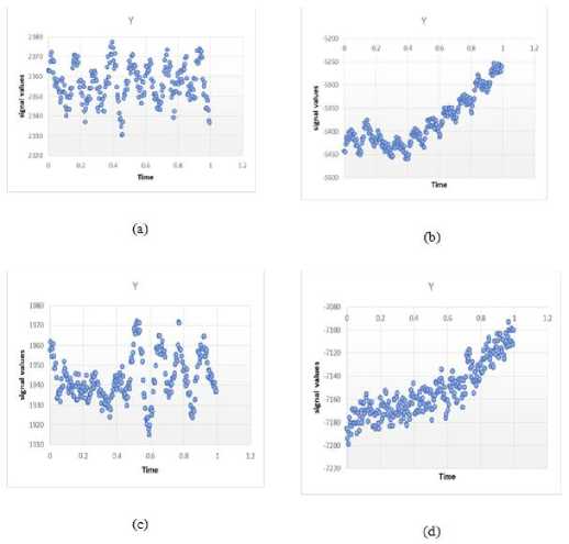
Fig.1. EEG print of channel Iz for one-second epoch

(a) Subject 3 epoch 1 eyes-opened, (b) Subject 21 epoch 1 eyes-opened, (c) Subject 3 epoch 1 eyes-closed, (d) Subject 21 epoch 1 eyes-closed

After that, a fusion of the three HjP with the 256-extracted samples for each epoch is applied. All the data were shuffled, then it was divided using a ten-fold cross-validation method, this method can guarantee unbiased performance measures.

To validate the performance of the proposed approach, we conducted four experiments: In experiment 1, classifiers were employed to the eyes-closed scenario without applying features fusion. In experiment 2, the authors employed the classification techniques to the eyes-closed after applying features fusion method. While in experiment 3, the eyes-opened scenario without applying the features fusion has executed. And finally, in experiment 4 the features fusion on the eyes-opened scenario has done.

The experiments are measured using five evaluators named, True Positive Rate (TPR), False Positive Rate (FPR), Precision, Recall and F-measure [51].

TPR = TP/(TP + FN)(5)

FPR = FP/(FP + TN)(6)

Precision = Confidence = TP/(TP + FP)

Recall = Sensitivity = TPR = TP/(TP + FN)

Fjneasnre = 2* Precision * Recall/ (Precision + Recall)

Where TP is True Positive, FN is False Negative, FP is False Positive and TN is True Negative.

4.1. Experiment 1
4.2. Experiment 2

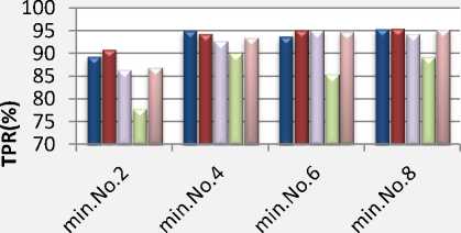
In the first experiment, we applied the proposed approach on the eyes-closed scenario without applying the fusion of the features. And we performed a comparison among the five tested classifiers as shown in figure 1.

As can be noticed, the results of RF classifier are the best and the most stable among the tested classifiers, which are; 91%, 94.3%, 95.2%, 95.5% for the four minutes respectively. But these results need more improvements to be applicable.

ы KNN и RF u NB □ SVM u DT

Time

Fig.2. Classifiers performance for each minute without features fusion

This experiment has been performed exactly as experiment1, but to improve the results, the authors proposed a features fusion level between the extracted samples of the EEG signal and the calculated HjP.

The best results are achieved using the KNN classifier as shown in table 1 and the results for the four minutes are 93.4%, 98.7%, 99.1% and 96% respectively.

Table 1.classifiers performance in experiment 2

	With features-fusion
	Min2	Min4	Min6	Min8
TPR	0.873	0.946	0.952	0.955
FPR	0.006	0.003	0.002	0.002
DT Precision	0.885	0.950	0.952	0.957
Recall	0.873	0.946	0.952	0.955
F-measure	0.871	0.945	0.951	0.949
TPR	0.883	0.924	0.907	0.907
FPR	0.006	0.004	0.005	0.005
SVM Precision	0.903	0.931	0.914	0.912
Recall	0.883	0.924	0.907	0.907
F-measure	0.882	0.921	0.906	0.905
TPR	0.874	0.928	0.954	0.944
FPR	0.006	0.004	0.002	0.003
NB Precision	0.883	0.928	0.959	0.936
Recall	0.874	0.928	0954	0.944
F-measure	0.871	0.926	0953	0.936
TP	0.918	0.950	0.954	0.959
FP	0.004	0.003	0.002	0.002
RF Precision	0.920	0.950	0.955	0.957
Recall	0.918	0.950	0.954	0.959
F-measure	0.917	0.950	0.953	0.957
TPR	0.934	0.987	0.991	0.960
FPR	0.003	0.001	0.000	0.002
KNN Precision	0.935	0.987	0.991	0.960
Recall	0.934	0.987	0.991	0.960
F-measure	0.934	0.987	0.991	0.959

The results show that the features fusion has achieved a considerable improvement to the performance of all the tested classifiers, for example, the accuracy of SVM at minute 2 is 78% without the features fusion while after the features level fusion, the results have achieved 88.3% and also the improvement for all the tested classifiers with different rates of improvement.

н KNN и RF □ NB и SVM U DT

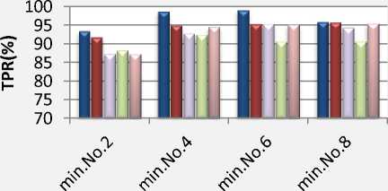
Fig.3. Classifiers performance for each minute with features fusion

Time

The comparison between the performance of the KNN classifier in the experiment1 and the experiment2 in figure 4 shows a significant improvement achieved in the experiment2; as the features-fusion improved the results of the KNN classifier for the four minutes with 4%, 3.7%, 5.4% and 0.6% respectively.

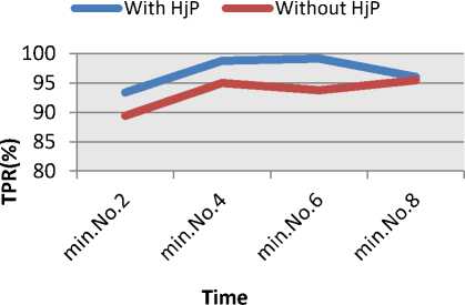
Fig.4. The effect of features fusion on the KNN classifier

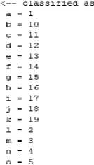
Tables 2,3,4,5 show the confusion matrices by the class of the proposed approach at minutes 2, 4, 6, 8. These matrices show that many subjects have been recognized with an accuracy of 100% (such as subjects: f, n, p, s and u) where the proposed approach has correctly recognized all the 58 epochs of them through the four minutes.

Table 2. The confusion matrix at min 2

=-= Confusion Matrix =-= abode f g h i j klmnopqrstu

56 00020000000000000000

0 58 0000000000000000000

00 49 000504000000000000

000 SS 00000000000000000 2000 56 0000000000000000

00000 58 000000000000000

006000 39 0 13 000000000000

0000000 57 0000000000010

006000 12 0 38 020000000000

000000000 58 00000000000

0000000010 57 0000000000

00000000000 58 000000000

000000000007 51 00000000

0000000000000 58 0000000

00000000000000 58 000000

000000000000000 5800000

0000000000000000 47 11000

00000000000000007 51000

000000000000000000 5800

0000000100000000000 570

00000000000000000000 58

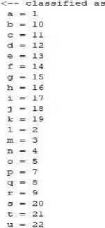
Table 3.The confusion matrix at min 4

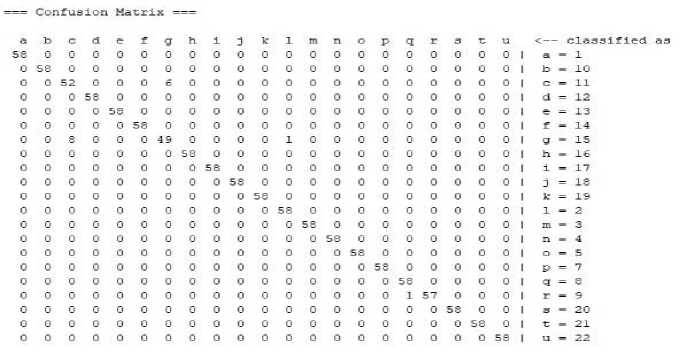
Table 4.The confusion matrix at min 6

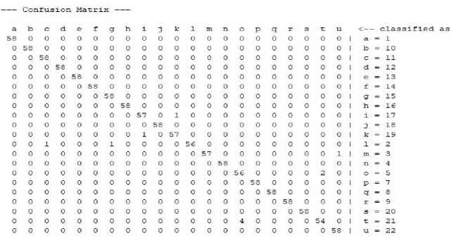
Table 5. The confusion matrix at min 8

=== Confusion Matrix

a	b	c	d	e	-	g	h		j		1	m	n	о	P	q	r	s	t	u		classified as
58	0	0	0	0	0	0	0	0	0	0	0	0	0	0	0	0	0	0	0	0	a	=	1
0	52	0	0	0	0	0	0	0	0	0	0	0	0	0	0	4	2	0	0	0	b	=	10
0	0	58	0	0	0	0	0	0	0	0	0	0	0	0	0	0	0	0	0	0	c	=	11
0	0	0	57	0	1	0	0	0	0	0	0	0	0	0	0	0	0	0	0	0	d	=	12
0	0	0	0	58	0	0	0	0	0	0	0	0	0	0	0	0	0	0	0	0	e	=	13
0	0	0	0	0	58	0	0	0	0	0	0	0	0	0	0	0	0	0	0	0	f	=	14
0	0	0	0	0	0	58	0	0	0	0	0	0	0	0	0	0	0	0	0	0	g	=	15
0	0	0	0	0	0	0	58	0	0	0	0	0	0	0	0	0	0	0	0	0	n	=	16
0	0	0	0	0	0	0	0	58	0	0	0	0	0	0	0	0	0	0	0	0		=	17
0	0	0	0	0	0	0	0	0	58	0	0	0	0	0	0	0	0	0	0	0	j	=	18
0	0	0	0	0	0	0	0	0	0	58	0	0	0	0	0	0	0	0	0	0	к	=	19
0	0	0	0	0	0	0	0	0	0	0	58	0	0	0	0	0	0	0	0	0	1	=	2
0	0	0	0	0	0	0	0	0	0	0	0	58	0	0	0	0	0	0	0	0	m	=	3
0	0	0	0	0	0	0	0	0	0	0	0	0	58	0	0	0	0	0	0	0	n	=	4
0	0	0	0	0	0	0	0	0	0	0	0	0	0	57	0	0	0	0	1	0	о	=	5
0	0	0	0	0	0	0	0	0	0	0	0	0	0	0	58	0	0	0	0	0	P	=	7
0	11	0	0	0	0	0	0	0	0	0	0	0	0	0	0	39		0	0	0	q	=	8
0	2	0	0	0	0	0	0	0	0	0	0	0	0	0	0	18	38	0	0	0	r	=	9
0	0	0	0	0	0	0	0	0	0	0	0	0	0	0	0	0	0	58	0	0	s	=	20
0	0	0	0	0	0	0	0	0	0	0	0	0	0	2	0	0	0	0	5€	0	t	=	21
0	0	0	0	0	0	0	0	0	0	0	0	0	0	0	0	0	0	0	0	58	u	=	22

4.3. Experiment 3
4.4. Experiment 4

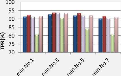
In this experiment, we applied the proposed approach on the eyes-opened scenario without applying the fusion of the features. And we performed a comparison among the five tested classifiers as shown in figure 5. As can be noticed, the results of RF classifier are the best and the most stable among the tested classifiers, which are; 92.5%, 93.8%, 93.5%, 91.8% for the four minutes respectively. But these results also need more improvements to be applicable.

н KNN и RF □ NB U SVM Li DT

Time

Fig.5. Classifiers performance for each minute without features fusion

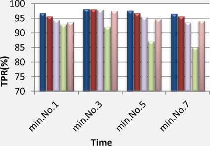
To improve the previous results, the authors proposed a features fusion level between the extracted samples of the EEG signal and the calculated HjP. The best results are achieved using the KNN classifier as shown in table 6 and the results for the four minutes are 96.8%, 98.2%, 97.7% and 96.6% respectively.

Table 6. Classifiers performance in experiment 4

	With features-fusion
	Min 1	Min 3	Min 5	Min 7
TPR	0.937	0.976	0.948	0.942
FPR	0.003	0.001	0.003	0.003
DT Precision	0.941	0.980	0.948	0.943
Recall	0.937	0.976	0.948	0.942
F-measure	0.936	0.975	0.948	0.941
TPR	0.929	0.921	0.872	0.851
FPR	0.004	0.004	0.006	0.007
SVM Precision	0.933	0.928	0.886	0.856
Recall	0.929	0.921	0.872	0.851
F-measure	0.929	0.920	0.867	0.843
TPR	0.945	0.979	0.955	0.937
FPR	0.003	0.001	0.002	0.003
NB Precision	0.948	0.980	0.958	0.939
Recall	0.945	0.979	0.955	0.937
F-measure	0.945	0.978	0.955	0.936
TPR	0.957	0.981	0.968	0.957
FPR	0.002	0.001	0.002	0.002
RF Precision	0.960	0.984	0.969	0.958
Recall	0.957	0.981	0.968	0.957
F-measure	0.957	0.981	0.968	0.957
TPR	0.968	0982	0.977	0.966
FPR	0.002	0.001	0.001	0.002
KNN Precision	0.968	0.983	0.977	0.967
Recall	0.968	0.982	0.977	0.966
F-measure	0.968	0.982	0.977	0.966

The comparison between results in figure 5 and results in figure 6 show that the features fusion has achieved a considerable improvement to the performance of all the tested classifiers.

н KNN и RF □ NB U SVM и DT

Fig.6. Classifiers performance for each minute with features fusion

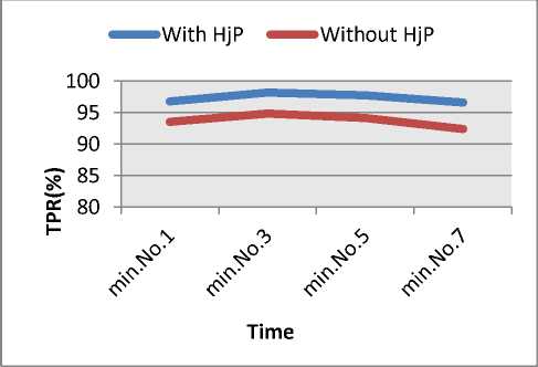
And the comparison between the performance of the KNN classifier in experiment 3 and experiment4 in figure 7 shows a significant improvement achieved in experiment 4; as the features-fusion improved the results of the KNN classifier for the four minutes with 3.3%, 3.4%, 3.6% and 4.2% respectively.

Fig.7. The effect of features fusion on the KNN classifier

Tables 7, 8, 9, 10 show the confusion matrices by the class of the proposed approach at minutes 1, 3, 5, 7. These matrices show that many subjects have been identified with an accuracy of 100%. Such as subjects: e, i, j, n, p and s.

Table 7. The confusion matrix at min 1

——— Confusion Matrix ——— abode f g h 58 0000000

0 57 000000 0 0 46 0 0 0 12 0 000 57 0000 0000 58 000 00000 58 00

0 0 11 0 0 0 47 0 0000000 54 00000000 00000000 00000000 00000000 00000000 00000000 00000001 00000000 04000000 00000000 00000000 00010001 00000000

i j к 1 m nо

0 0 0 0 0 00

0 0 0 0 0 02

58 0 0 0 0 00

0 58 0 0 0 00

0 0 58 0 0 00

0 0 0 57 0 00

0 0 0 0 56 00

0 0 0 0 0 580

0 0 0 0 0 057

0 0 0 0 0 00

0 0 0 2 0 00

0 0 0 0 00

0 1 0 0 00

0 0 0 0 00

0 0 0 0 10

0 0 0 0 00

0 0 0 0 20

0 0 0 0 00

0 0 0 0 01

0 0 0 0 00

58 0 0 0 00

0 54 0 0 00

0 0 58 0 00

0 0 0 58 00

0 0 0 0 560

0 0 0 0 056

Table 8. The confusion matrix at min 3

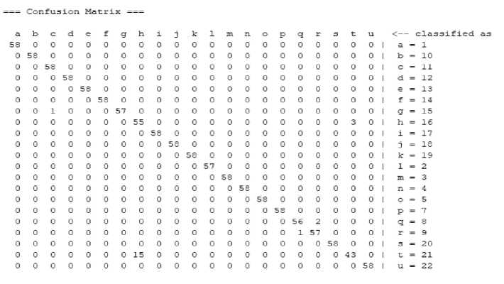
Table 9. The confusion matrix at min 5

= Confusion Matrix

a	b	c	d	€	f	g	h	1	3	к	1	m	n	о	p	q	r	3		u	<— classified, as
58	0	0	0	0	0	0	0	0	0	0	0	0	0	0	0	0	0	0	0	0 I	a = 1
0	58	0	0	0	0	0	0	0	0	0	0	0	0	0	0	0	0	0	0	0 I	b = 10
0	0	46	0	0	0	11	0	0	0	0	1	0	0	0	0	0	0	0	0	0 I	c = 11
0	0	0	58	0	0	0	0	0	0	0	0	0	0	0	0	0	0	0	0	0 I	d = 12
0	0	0	0	58	0	0	0	0	0	0	0	0	0	0	0	0	0	0	0	0 I	e = 13
0	0	0	0	0	58	0	0	0	0	0	0	0	0	0	0	0	0	0	0	0 I	f = 14
0	0	:	0	0	0	50	0	0	0	0	0	0	0	0	0	0	0	0	0	0 I	g = 15
0	0	0	0	0	0	0	53	0	0	0	0	0	0	0	0	0	0	0	0	0 I	h = 16
0	0	0	0	0	0	0	0	58	0	0	0	0	0	0	0	0	0	0	0	0 1	i = 17
0	0	0	0	0	0	0	0	0	53	0	0	0	0	0	0	0	0	0	0	0 I	j = 18
0	0	0	0	0	0	0	0	1	0	57	0	0	0	0	0	0	0	0	0	0 I	к = 19
0	0	0	0	0	0	0	0	0	0	0	58	0	0	0	0	0	0	0	0	0 I	1 = 2
0	0	0	0	0	0	0	0	0	0	0	0	56	0	0	0	0	0	0	0	2 I	m = 3
0	0	0	0	0	0	0	0	0	0	0	0	0	58	0	0	0	0	0	0	0 I	n = 4
0	0	0	0	0	0	0	0	0	0	0	0	0	0	58	0	0	0	0	0	0 I	o = 5
0	0	0	0	0	0	0	0	0	0	0	0	0	0	0	58	0	0	0	0	0 I	p = 7
0	0	0	0	0	0	0	0	0	0	0	0	0	0	0	0	58	0	0	0	0 I	q = 8
0	0	0	0	0	0	0	0	0	0	0	0	0	0	0	0	0	58	0	0	0 I	r = 9
0	0	0	0	0	0	0	0	0	0	0	0	0	0	0	0	0	0	58	0	0 I	s = 20
0	0	0	0	0	0	0	1	0	0	0	0	0	0	2	0	0	0	0	55	0 I	t = 21
0	0	0	0	0	0	0	0	0	0	0	0	0	0	0	0	0	0	0	0	58 1	u = 22

Table 10. The confusion matrix at min 7

— Confusion Matrix ——— a b c d e fg

57 0 0 0 0 00

0 55 0 0 0 00

0 0 58 0 0 00

0 0 0 55 0 10

0 0 0 0 58 00

0 0 0 3 0 500

0 0 0 0 0 057

0 0 0 4 0 60

0 0 0 0 0 00

0 2 0 0 0 00

0 0 0 0 0 00

b 1 3 к 1 m n о

00000000 00000000

00000000 20000000 00000000 50000000 00001000

48 0000000

0 58 000000

00 5800000

000 580000

0 00 0 58000

00000 5800

000000 580

0000000 57 00000000 00000000 00000000 00000000 00000005 00000000

p q Г s tU

0 0 0 0 00

0 0 3 0 00

0 0 0 0 00

0 0 0 0 10

58 0 0 0 00

0 52 6 0 00

0 2 54 0 00

0 0 0 58 00

0 0 0 0 530

0 0 0 0 058

P = 7

q = 8

5. Conclusions and Future Work

This study has focused on developing a new approach to human recognition utilizing EEG signals. The main contribution of this study is optimizing the time needed for capturing the signal to one-second only, extracted using only single-channel. The uniqueness of our proposed method relies on the features-fusion level between the signal and the Hjorth parameters. We emphasized the proposed technique by testing on a public dataset in the two different states of resting. We conducted a comparison among five different classifiers’ performance without and with using the proposed technique and the results show the improvement in the performance of all the tested classifiers. The results proved the proposed approach constancy for all the subjects, achieving TPR of 100% for multiple subjects and average True Positive Rate (TPR) 99.1% for eyes-closed scenario and 98.2% for eyes-opened scenario. In the future, large datasets will be tested and also data acquired from the wearable EEG devices.

Список литературы A Biometric System Based on Single-channel EEG Recording in One-second

M. P. ; M. R. ; V. C. ; A. Evangelou, “PERSON IDENTIFICATION BASED ON PARAMETRIC PROCESSING OF THE EEG,” 1999.
M. Abo-Zahhad, S. M. Ahmed, and S. N. Abbas, “A new multi-level approach to EEG based human authentication using eye blinking,” Pattern Recognit. Lett., vol. 82, pp. 216–225, 2016.
C. Rig Das, Maiorana, “EEG Biometrics Using Visual Stimuli : a Longitudinal Study,” IEEE Signal Process. Lett. Vol. Issue 3, vol. 9908, no. c, pp. 1–9, 2016.
Z. A. Alkareem Alyasseri, A. T. Khader, M. A. Al-Betar, J. P. Papa, O. A. Alomari, and S. N. Makhadme, “An efficient optimization technique of EEG decomposition for user authentication system,” 2nd Int. Conf. BioSignal Anal. Process. Syst. ICBAPS 2018, pp. 1–6, 2018.
L. A. Moctezuma, A. A. Torres-García, L. Villaseñor-Pineda, and M. Carrillo, “Subjects identification using EEG-recorded imagined speech,” Expert Syst. Appl., vol. 118, pp. 201–208, 2019.
S. Marcel and J. del R. Millan, “Person authentication using brainwaves (EEG) and maximum a posteriori model adaptation,” IEEE Trans. Pattern Anal. Mach. Intell., vol. 29, no. 4, pp. 743–748, 2007.
E. S. Haukipuro et al., “Mobile brainwaves: On the interchangeability of simple authentication tasks with low-cost, single-electrode EEG devices,” IEICE Trans. Commun., vol. E102B, no. 4, pp. 760–767, 2019.
P. Campisi and D. La Rocca, “Brain waves for automatic biometric-based user recognition,” IEEE Trans. Inf. Forensics Secur., vol. 9, no. 5, pp. 782–800, 2014.
R. Suppiah and A. P. Vinod, “Biometric identification using single channel EEG during relaxed resting state,” IET Biom., vol. 7, pp. 342–348, 2018.
M. Hunter et al., “The Australian EEG Database,” Clin. EEG Neurosci., vol. 36, no. 2, pp. 76–81, 2005.
“The CSU EEG database.” [Online]. Available: http://www.cs.colostate.edu/eeg/main/data/2011-12_BCI_at_CSU. [Accessed: 17-Jul-2019].
“EEG During Mental Arithmetic Tasks.” [Online]. Available: https://physionet.org/physiobank/database/eegmat/[Accessed:17-Jul-2019].
“EEG Motor Movement/Imagery Dataset.” [Online]. Available: https://physionet.org/physiobank/database/eegmmidb/ [Accessed:17-Jul-2019].
“EEG Signals from an RSVP Task.” [Online]. Available: https://physionet.org/physiobank/database/ltrsvp/ [Accessed:17-Jul-019].
“ERP-based Brain-Computer Interface recordings.” [Online]. Available: https://physionet.org/physiobank/database/erpbci/ [Accessed:17-Jul-019].
“Evoked Auditory Responses in Normals across Stimulus Level.” [Online]. Available: https://physionet.org/physiobank/database/earndb/ [Accessed:17-Jul-019].
“MAMEM Steady State Visually Evoked Potential EEG Database.”[Online].Available: https://physionet.org/physiobank/database/mssvepdb/ [Accessed:17-Jul-2019].
“Deap dataset.”[Online]. Available: http://www.eecs.qmul.ac.uk/mmv/datasets/deap/index.html [Accessed:17-Jul-019].
“The UCI EEG dataset.” [Online]. Available: https://archive.ics.uci.edu/ml/datasets/eeg%2Bdatabase [Accessed:17-Jul-2019].
“Texas Data Repository.” [Online]. Available: https://dataverse.tdl.org/dataset.xhtml?persistentId=doi:10.18738/T8/9TTLK8 [Accessed:17-Jul-2019].
C. Brunner and R. Leeb, “Graz_Bci dataset A,” pp. 1–6, 2008.
G. P. Clemens Brunner, Robert Leeb, Gernot Müller-Putz, Alois Schlögl, “BCI Competition 2008 – Graz data set B,” Knowl. Creat. Diffus. Util., pp. 1–6, 2008.
“ATR dataset.” [Online]. Available: https://biomark00.atr.jp/modules/xoonips/listitem.php?indexid=181 [Accessed:17-Jul-019].
“Keirn_and_Aunon dataset.” [Online]. Available: http://www.cs.colostate.edu/eeg/main/data/1989_Keirn_and_Aunon [Accessed:17-Jul-019].
“Benci dataset.” [Online]. Available: http://bnci-horizon-2020.eu/database/data-sets [Accessed:17-Jul-019].
G. Q. Zhu Dan, Zhou Xifeng, “An Identification System Based on Portable EEG Acquisition Equipment,” in Third International Conference on Intelligent System Design and Engineering Applications, 2013.
Y. Bai, Z. Zhang, and D. Ming, “Feature selection and channel optimization for biometric identification based on visual evoked potentials,” in 19th International Conference on Digital Signal Processing, 2014, no. August, pp. 772–776.
S. Keshishzadeh and A. Fallah, “Improved EEG based human authentication system on large dataset,” in Iranian Conference on Electrical Engineering (ICEE), 2016, pp. 1165–1169.
L. A. Moctezuma, A. A. Torres-garc, L. Villase, L. A. Moctezuma, and A. A. Torres-garc, “Subjects Identification using EEG-recorded Imagined Speech,” Expert Syst. With Appl. Elsevier, 2018.
Y. Sun, F. P. Lo, and B. Lo, “EEG-based user identification system using 1D-convolutional long short-term memory neural networks,” Expert Syst. Appl., 2019.
S. Liu et al., “Individual Feature Extraction and Identification on EEG Signals in Relax and Visual Evoked Tasks,” in Biomedical Informatics and Technology, 2014, pp. 305–318.
P. Nguyen, D. Tran, X. Huang, and D. Sharma, “A Proposed Feature Extraction Method for EEG-based Person Identification,” Int. Conf. Artif. Intell., 2012.
S. K. Yeom, H. Il Suk, and S. W. Lee, “Person authentication from neural activity of face-specific visual self-representation,” Pattern Recognit., vol. 46, no. 4, pp. 1159–1169, 2013.
Q. Gui, Z. Jin, and W. Xu, “Exploring EEG-based biometrics for user identification and authentication,” 2014 IEEE Signal Process. Med. Biol. Symp. IEEE SPMB 2014 - Proc., 2015.
F. Su, L. Xia, A. Cai, Y. Wu, and J. Ma, “EEG-based personal identification: From proof-of-concept to a practical system,” Proc. - Int. Conf. Pattern Recognit., pp. 3728–3731, 2010.
M. K. Abdullah, K. S. Subari, J. L. C. Loong, and N. N. Ahmad, “Analysis of effective channel placement for an EEG-based biometric system,” Proc. 2010 IEEE EMBS Conf. Biomed. Eng. Sci. IECBES 2010, no. December, pp. 303–306, 2010.
B. Kaur, P. Kumar, P. P. Roy, and D. Singh, “Impact of Ageing on EEG based Biometric Systems,” 2017 4th IAPR Asian Conf. Pattern Recognit., pp. 459–464, 2017.
W. Rahman and M. Gavrilova, “Overt Mental Stimuli of Brain Signal for Person Identification,” in International Conference on Cyberworlds, 2016, pp. 197–203.
C. M. Issac and E. G. M. Kanaga, “Probing on Classification Algorithms and Features of Brain Signals Suitable for Cancelable Biometric Authentication,” 2017 IEEE Int. Conf. Comput. Intell. Comput. Res., pp. 1–4, 2017.
K. Bashar, “ECG and EEG Based Multimodal Biometrics for Human Identification,” 2018 IEEE Int. Conf. Syst. Man, Cybern., pp. 4345–4350, 2018.
[41]J. Chuang, H. Nguyen, C. Wang, and B. Johnson, “I Think, Therefore I Am: Usability and Security of Authentication Using Brainwaves,” in Financial Cryptography and Data Security, 2013, pp. 1–16.
M. T. Curran, J. K. Yang, N. Merrill, and J. Chuang, “Passthoughts authentication with low cost EarEEG,” Proc. Annu. Int. Conf. IEEE Eng. Med. Biol. Soc. EMBS, vol. 2016-Octob, pp. 1979–1982, 2016.
Z. Liang, S. Oba, and S. Ishii, “An Unsupervised EEG Decoding System for Human Emotion Recognition Acknowledgments This study was supported by the New Energy and Industrial Technology Development,” Neural Networks, 2019.
A. Patil, “FEATURE EXTRACTION OF EEG FOR EMOTION RECOGNITION USING HJORTH FEATURES AND HIGHER ORDER CROSSINGS,” in Conference on Advances in Signal Processing (CASP) Cummins College of Engineering for Women, Pune., 2016, pp. 429–434.
O. O. Kübra Eroğlu, Pınar Kurt, Temel Kayıkçıoğlu, “Investigation of Luminance Effect on the Emotional Assessment Using Hjorth Descriptors,” in Medical Technologies National Congress (TIPTEKNO), 2016
M. Tanveer, “Classification of seizure and seizure-free EEG signals using Hjorth parameters,” in 2018 IEEE Symposium Series on Computational Intelligence (SSCI), 2018, pp. 2180–2185.
R. M. Mehmood, R. Du, and H. J. Lee, “Optimal feature selection and deep learning ensembles method for emotion recognition from human brain EEG sensors,” IEEE Access, vol. 5, pp. 14797–14806, 2017.
S.-H. Liew, Y.-H. Choo, Y. F. Low, and Z. I. Mohd Yusoh, “EEG-based biometric authentication modelling using incremental fuzzy-rough nearest neighbour technique,” IET Biometrics, vol. 7, no. 2, pp. 145–152, 2017.
E. Frank, M. A. Hall, and I. H. Witten, “The WEKA Workbench Data Mining: Practical Machine Learning Tools and Techniques,” Morgan Kaufmann, Fourth Ed., p. 128, 2016.
A. Delorme and S. Makeig, “EEGLAB: an open source toolbox for analysis of single-trial EEG dynamics including independent component analysis,” vol. 134, pp. 9–21, 2004.
POWERS, D.M.W., " EVALUATION: FROM PRRECISION, RECALL AND F-MEASURE TO ROC, INFORMEDNESS, MARKEDNESS & CORRELATION", Journal of Machine Learning Technologies, Volume 2, Issue 1, 2011, pp-37-63

Еще

Статья научная