A Comparison of BA, GA, PSO, BP and LM for Training Feed forward Neural Networks in e-Learning Context

Published Online June 2012 in MECS

Optimization has been an active area of research for several decades. As many real-world optimization problems become more complex, better optimization algorithms were needed. In all optimization problems the goal is to find the minimum or maximum of the objective function. Thus, unconstrained optimization problems can be formulated as minimization or maximization of D dimensional function:

Min (or max) f(x), x=(x 1 , x 2 , x 3,…, x D )             (1)

where D is the number of parameters to be optimized.

Many population based algorithms were proposed for solving unconstrained optimization problems. Genetic algorithms (GA), particle swarm optimization (PSO), and bat algorithms (BA) are most popular optimization algorithms which employ a population of individuals to solve the problem on hand. The success or failure of a population based algorithms depends on its ability to establish proper trade-off between exploration and exploitation. A poor balance between exploration and exploitation may result in a weak optimization method which may suffer from premature convergence, trapping in a local optima and stagnation.

GA is one of the most popular evolutionary algorithms in which a population of individuals evolves (moves through the fitness landscape) according to a set of rules such as selection, crossover and mutation [1].

PSO algorithm is another example of population based algorithms [2]. PSO is a stochastic optimization technique which is well adapted to the optimization of nonlinear functions in multidimensional space and it has been applied to several real-world problems [3].

BA is a relatively new population based metaheuristic approach based on hunting behavior of bats [8]. In this algorithm possible solution of the problem is represented by bat positions. Quality of the solution is indicated by the best position of a bat to its prey. BA has been tested for continuous constrained optimization problems [23].

The interest of the research in Artificial Neural Networks (ANNs) resides in the appealing properties they exhibit: adaptability, learning capability, and ability to generalize. Nowadays, ANNs are receiving a lot of attention from the international research community with a large number of studies concerning training, structure design, and real world applications, ranging from classification to robot control or vision [1]. Feed-forward neural networks (NNs) are popular classification tools. Each feed-forward NN consists of an input layer of neurons. In case of the classification problem the input layer consists of as many neurons as there are measurements in the patterns, that is, for each measurement there exists exactly one input neuron. Furthermore, a feed-forward NN consists of an arbitrary number of hidden layers of neurons, and an output layer (cf. Figure 1).

The outline of this paper is as follows. Section II describes the different types of metaheuristics used in this paper, two artificial neural network metaheuristics, 1) gradient-descent algorithm, and 2) Levenberg-Marquardt backpropaction algorithm, three population based methheuristics 1) genetic algorithm, 2) particle swarm algorithm, and 3) bat algorithm. In Section III, benchmarking testing and elearning datasets are described together with the performance analysis of the test results. Most importantly the parameters for the algorithms are given for the individual tests. Section IV presents conclusions and final comments.

• II.    Metaheuristics

Metaheuristics have been established as one of the most practical approach to simulation optimization. However, these methods are generally designed for combinatorial optimization, and their implementations do not always adequately account for the presence of simulation noise.

Research in simulation optimization, on the other hand, has focused on convergent algorithms, giving rise to the impression of a gap between research and practice. This paper surveys the use of metaheuristics for simulation optimization, focusing on work bridging the current gap between the practical use of such methods and research, and points out some promising directions for research in this area. The main emphasis is on two issues: accounting for simulation noise in the implementation of metaheuristics, and convergence analysis of metaheuristics that is both rigorous and of practical value. To illustrate the key points, metaheuristics are discussed and used, namely artificial neural networks, Levenberg-Marquardt search algorithm, genetic algorithm, particle swarm optimization, and the bat algorithm.

• A.    Artificial Neural Networks (ANNs)

The backpropagation algorithm (BP) [2] is a classical domain-dependent technique for supervised training (cf. Figure 1). It works by measuring the output error, calculating the gradient of this error, and adjusting the ANN weights (and biases) in the descending gradient direction.

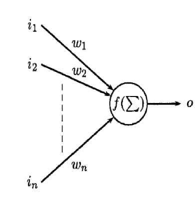
Figure 1. ANN Neuron

Hence, BP is a gradient-descent local search procedure (expected to stagnate in local optima in complex landscapes). The squared error of the ANN for a set of patterns is:

Е= ∑Р=1 ∑7=1( if - о- ) (2)

The actual value of the previous expression depends on the weights of the network. The basic BP algorithm calculates the gradient of E (for all the patterns) and updates the weights by moving them along the gradientdescendent direction. This can be summarized with the expression ∆w = -η∇E, where the parameter η > 0 is the learning rate that controls the learning speed. The pseudo-code of the BP algorithm is shown (cf. Figure 2).

Initialize Weights;

While not Stop-Criterion do

For all i, j do

ЭЕ

Wit =    - η

End For

End While

Figure 2. Pseudocode of backpropagation algorithm

• B.    Levenberg-Marquardt

The Levenberg-Marquardt algorithm (LM) [9] is an approximation to the Newton method (cf. Figure 3) used also for training ANNs.

Neural Networks in e-Learning Context

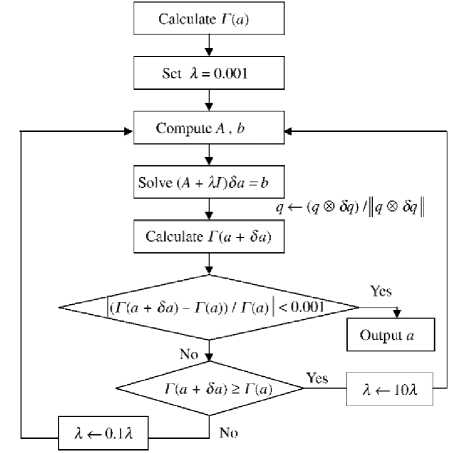
Figure 3. Flow chart of Levenberg-Marquardt

The Newton method approximates the error of the network with a second order expression, which contrasts to the Backpropagation algorithm that does it with a first order expression. LM updates the ANN weights as follows:

Aw = [ц1 + E =iF(wY p(w]V ^(w)    (3)

Where Jp (w) is the Jacobian matrix of the error vector ep (w) evaluated in w, and I is the identity matrix. The vector error ep (w) is the error of the network for pattern p, that is, ep (w) = tp -op (w). The parameter µ is increased or decreased at each step. If the error is reduced, then µ is divided by a factor β, and it is multiplied by β in other case. Levenberg-Marquardt performs the steps detailed in Fig. 3. It calculates the network output, the error vectors, and the Jacobian matrix for each pattern. Then, it computes ∆w using (3) and recalculates the error with w + ∆w as network weights. If the error has decreased, µ is divided by β, the new weights are maintained, and the process starts again; otherwise, µ is multiplied by β, ∆w is calculated with a new value, and it iterates again.

Initialize Weights;

While not Stop-Criterion do

Calculates c^p(w) for each pattern e i = Zp = i e^p(w^)T e^p(w)

Calculates Jp(w) for each pattern

Repeat

Calculates Aw

e2 = Ep = 1ep(w + Aw) ep(w + Aw)

If e1 ≤ e2 Then μ = μ * β end If

Until e1 < e2

μ = μ/β w = w + ∆w

End While

• Figure 4. Pseudocode of Levenberg-Marquardt algorithm

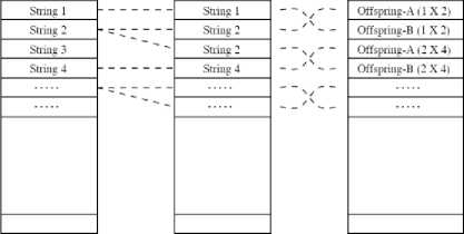
• C.    Genetic Algorithm (GA)

A GA [12] is a stochastic general search method. It proceeds in an iterative manner by generating new populations of individuals from the old ones (cf. Figure 4). Every individual is the encoded (binary, real, etc.) version of a tentative solution. Figure 5 shows the selection and recombination phases of the genetic algorithm.

Recombination (Crossover)

Selection (Duplication)

Current                Intermediate                  Next

Generation t             Generation t            Generation t + 1

Figure 5. Selection and recombination phase of the genetic algorithm

The canonical algorithm applies stochastic operators such as selection, crossover, and mutation on an initially random population in order to compute a new population. In generational GAs all the population is replaced with new individuals. In steady-state GAs (used in this work) only one new individual is created and it replaces the worst one in the population if it is better. The pseudo-code of the GA we are using here can be seen in Fig. 4. The search features of the GA contrast with those of the BP and LM in that it is not trajectory-driven, but population-driven. The GA is expected to avoid local optima frequently by promoting exploration of the search space, in opposition to the exploitative trend usually allocated to local search algorithms like BP or LM. The pseudocode for the genetic algorithm is shown on Figure 6.

t = 0

Initialize: P(0) = {a i (0), ..., a ^ (0)} e F

Evaluate: P(0): {Φ(a 1 (0)), …, Φ(a μ (0))}

While £ (P(t)) ^ true //Reproductive loop

Select: P’(t) = s θz {P(t)}

Recombine: P’’(t) = ®8z {P’(t)}

Mutate: P’’’(t) = m θm {P’’(t)}

Evaluate: P’’’(t): {Φ(a 1 ^’’’(t)), …, Φ(a λ ^’’’(t))}

Replace: P(t+1) = r ^r (P’’’(t) U Q)

t = t + 1

End While

• Figure 6. Pseudocode of genetic algorithm

• D.    Particle Swarm Optimization (PSO)

The PSO algorithm was first introduced by Eberhart and Kennedy [5, 6, 7, and 8]. Instead of using evolutionary operators to manipulate the individuals, like in other evolutionary computational algorithms, each individual in PSO flies in the search space with a velocity which is dynamically adjusted according to its own flying experience and its companions’ flying experience. Each individual is treated as a volume-less particle (a point) in the D-dimensional search space (cf. Figure 7).

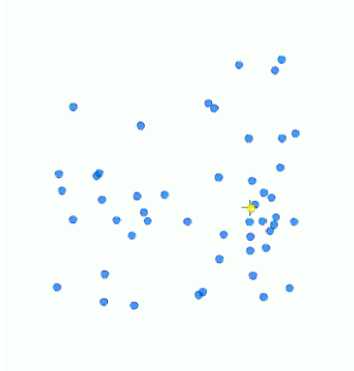
Figure 7. Particles movement in PSO

The ith particle is represented as X_i = (x_il, x_i2, ..., x_iD). The best previous position (the position giving the best fitness value) of the ith particle is recorded and represented as P i = (p il , p i2 , ..., p iD ). The index of the best particle among all the particles in the population is represented by the symbol gb representing global best. The index of the best position for each particle in the population is represented by the symbol ib representing the individual’s best. The rate of the position change (velocity) for particle i is represented as V i to the following equation: (v_il, v_i2, ..., v_iD). The particles are manipulated according to the following equations:

vtd = vt_d + c₁ * ran (() * ⁽p _tb -x_td ) + c ₂ * ran(.Q *

(Pgь - x_ta)                                           (4)

xtd = x_td + Vid                                     (5)

The algorithm can be summarized as follows:

Step1 Initialize position and velocity of all the particles randomly in the N dimension space.

Step2 Evaluate the fitness value of each particle, and update the global optimum position.

Step3 According to changing of the gathering degree and the steady degree of particle swarm, determine whether all the particles are re-initialized or not.

Step4 Determine the individual best fitness value. Compare the p of every individual with its current fitness value. If the current fitness value is better, assign the current fitness value to p . i

Step5 Determine the current best fitness value in the entire population. If the current best fitness value is better than the p , assign the current best fitness value to p .

g

Step6 For each particle, update particle velocity,

Step7 Update particle position.

Step8 Repeat Step 2 - 7 until a stop criterion is satisfied or a predefined number of iterations are completed.

The particle swarm flowchart is shown on Figure 8.

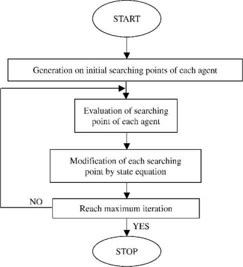
Figure 8. PSO Flowchart

• E.    Bat Algorithm (BA)

The bat algorithm [23] uses the echolocation behaviour of bats (cf. Figure 9). These bats emit a very loud sound pulse (echolocation) and listens for the echo that bounces back from the surrounding objects (cf. Figure 7). Their signal bandwidth varies depending on the species, and increases using harmonics. The ith bat flies randomly with velocity v i at position X i with a fixed frequency f_min. The bat varies its wavelength λ and loudness A 0 to search for food.

Figure 9. Micro-bat hunting for prey using echolocation

Neural Networks in e-Learning Context

The number of bats is n b .

f = ft = fmin + (fmax - fmin) 5

v =v + (X -Х   ) f(8)

It is assumed that the loudness varies from a large (positive) A 0 to a minimum constant value A min . The new solutions of the ith bat at time step t are given by X i ^t and v i ^t.

X =X + v                              (9)

where 5 [0, 1] is a random vector drawn from a uniform distribution. The domain size of the problem in context determines the values of f_min and f_max. Initially, each bat is randomly assigned a frequency which is drawn uniformly from [f min , f max ]. For local search procedure (exploitation) each bat takes a random walk creating a new solution for itself based on the best selected current solution.

X =X + ρΑ                              (10)

where   [-1,1] is a random number, At is the average loudness of all bats at this time step. The loudness decreases as a bat tends closer to its food and pulse emissions rate increases.

A =αΑ                                  (11)

r =r [1-е  ]                                (12)

where (comparative to the cooling factor of schedule in simulated annealing) and are constants.

• III.    Benchmarking Testing and e-Learning Datasets

Proben1 is a collection of problems for neural network learning in the realm of pattern classification and function approximation plus a set of rules and conventions for carrying out benchmark tests with these or similar problems. Proben1 contains 15 data sets from 12 different domains. All datasets represent realistic problems which could be called diagnosis tasks and all but one consist of real world data. The datasets are all presented in the same simple format, using an attribute representation that can directly be used for neural network training. Along with the datasets, Proben1 defines a set of rules for how to conduct and how to document neural network benchmarking. The purpose of the problem and rule collection is to give researchers easy access to data for the evaluation of their algorithms and networks and to make direct comparison of the published results feasible [18].

• A.    Standard datasets

We chose three problems from the well-known Proben1 benchmark set (cf. Table 1). The standard Proben1 benchmarking rules were applied [18]. Datasets were used with even-numbered examples used for the training set and odd-numbered examples used for the test set.

Table 1 Standard Datasets

Dataset	Number of patterns	Number of parameters	Number of outputs	Classification
Cancer 1st dataset	699	9	2	Pathological or normal
Diabetes 1st dataset	768	8	2	Pathological or normal
Heart 1st dataset	920	35	2	Pathological or normal
Thyroid 1st dataset	7200	21	3	Hyper of hypo function

• B.    Elearning datset

A group of medical students were tested using a medical health application. Students were given one hour to complete the eLearning tasks and complete a set of questions online. Ninety students participated in the experiment. Six students were tested thoroughly in the Usability Lab. The average time taken to complete the tasks were 48 minutes and the average percentage of correct questions was 76 percent.

Table 2 Elearning Datasets

Dataset	Number of patterns	Number of parameters	Number of outputs	Classificati on
eLearni ng	90	5	2	Bad or Good design

• C.    Results and algorithm’s settings

The mean squared error function was used as the training error. For all population based algorithms the population size was set at 30 [23]. This was done to uniformly survey the performance of the algorithms without too much variation. The parameters for the genetic algorithm were mutation rate=0.001, crossover rate=0.7 with the selection method being uniform (suitably fit members are chosen to breed at random) and crossover method is single-point (parents' genes are swapped over at one point along their length) [5]. The two constants for the PSO algorithm were given values of 2 [5]. The bat algorithm used the following settings: A0 = 1.0, Amin = 0.0, r0i = 0.01, α= γ=0.6 [23]. The learning rate of the steepest decent and Levenberg-Marquardt back-propagation algorithms were set to 0.3 [18]. Each run stops either when the error obtained is less than 10-8, or when the maximal number of evaluations (100 000) is achieved. All tests were carried out on a 64-bit operating system with a 2.4GHz CPU and 2GB RAM. Table 1 shows the average number of function evaluations obtained for each algorithm for each of the benchmark datasets considered. Table 2 shows the average error obtained for each algorithm for each of the benchmark datasets considered. Best performances are highlighted in both tables.

Table 3 Average number of function evaluations

Dataset	Average number of function evaluations
	NN-BP	NN-LM	NN-GA	NN-PSO	NN-BA
Heart 1	150948	2531	2867	2502	2432
Thyroid 1	1460835	61306	52990	56400	43514
Cancer 1	261	996	979	643	206
Diabetes 1	20675	1562	1203	1697	759
eLearning	8534	1535	765	2561	614

Table 4 Average error

Dataset	Average error
	NN-BP	NN-LM	NN-GA	NN-PSO	NN-BA
Cancer 1	3.24e-4	2.27e-5	2.05e-5	4.21e-5	1.99e-5
Diabetes 1	2.21e-4	7.39e-5	9.67e-5	1.80e-5	2.15e-5
Heart 1	5.32e-5	1.55e-5	4.21e-5	1.94e-5	2.58e-6
Thyroid 1	1.1e-5	2.77e-5	3.59e-5	2.42e-5	5.93e-6
eLearning	8.46e-5	3.15e-6	1.33e-5	3.19e-5	3.12e-6

The bat algorithm incorporates a combination of particle swarm optimization (PSO), harmony search (HS) and simulated annealing (SA) using a certain combination of parameters. The results clearly show that the combination of these algorithms into the bat algorithm enhances its performance as an optimization algorithm under different conditions. This is shown by the fact that for all the test datasets the BA outperforms the other algorithms. However, it is noted that in some cases the improvements are only minimal.

• IV.    Conclusions

A comparison of algorithms for training feed forward neural networks was done. Tests were done on two gradient descent algorithms: Backpropagation and Levenberg-Marquardt, and three population based heuristic: Bat Algorithm, Genetic Algorithm, and Particle Swarm Optimization. Experimental results show that bat algorithm (BA) outperforms all other algorithms in training feed forward neural networks. It supports the usage of the BA in further experiments and in further real world applications.

In this study, the Bat Algorithm (BA) Algorithm, which is a new, simple and robust optimization algorithm, has been used to train standard and eLearning datasets for classification purposes. First, well-known classification problems obtained from Proben1 [18] repository have been used for comparison. Then, an experimental setup has been designed for an eLearning based on health classification. Training procedures involves selecting the optimal values of the parameters such as weights between the hidden layer and the output layer, spread parameters of the hidden layer base function, center vectors of the hidden layer and bias parameters of the neurons of the output layer.

Trapping a local minimum is a disadvantage for these algorithms. The GA and ABC algorithms are population based evolutional heuristic optimization algorithms. These algorithms show better performance than derivative based methods for well known classification problems such as Iris, Glass, and Wine and also for experimental eLearning based health classification. However, these algorithms have the disadvantage of a slow convergence rate. If the classification performances are compared, experimental results show that the performance of the BA algorithm is better than those of the others.

The success of the classification results of test problems are superior and also correlates with the results of many papers in the literature. In real-time applications, number of neurons may affect the time complexity of the system. The results of eLearning classification problem are reasonable and may help to the planning algorithms in other eLearning applications.