A Comparison of Crowding Differential Evolution Algorithms for Multimodal Optimization Problems

Автор: O. Tolga Altinoz

Журнал: International Journal of Intelligent Systems and Applications(IJISA) @ijisa

Статья в выпуске: 4 vol.7, 2015 года.

Бесплатный доступ

Multimodal problems are related to locating multiple, redundant global optima, as opposed to single solution. In practice, generally in engineering problems it is desired to obtain many redundant solutions instead of single global optima since the available resources cannot be enough or not possible to implement the solution in real-life. Hence, as a toolbox for finding multimodal solutions, modified single objective algorithms can able to use. As one of the fundamental modification, from one of the niching schemes, crowding method was applied to Differential Evolution (DE) algorithm to solve multimodal problems and frequently preferred to compared with developed methods. Therefore, in this study, eight different DE are considered/evaluated on ten benchmark problems to provide best possible DE algorithm for crowding operation. In conclusion, the results show that the time varying scale mutation DE algorithm outperforms against other DE algorithms on benchmark problems.

Еще

Differential Evolution, Random Scale, Multimodal Optimization, Time Varying, Crowding

Короткий адрес: https://sciup.org/15010671

IDR: 15010671

Текст научной статьи A Comparison of Crowding Differential Evolution Algorithms for Multimodal Optimization Problems

Published Online March 2015 in MECS

The optimization problems are generally contains many local and global optimum points. For applications like function optimization, only the single global optimum point is desired to find by optimization algorithms since the aim of optimization algorithms is to minimize the cost function. However, in general, many of engineering problems may contain many redundant solutions which have the same cost value. Similarly, for some real-life problems, a single best-possible solution is needed to obtain in design stage. However, for practice perspective, it isn't convenient to find a single solution since the problem cannot be able to materialize due to physical and manufacture constraints [1]. Therefore, instead of a single solution, other redundant solutions are desired to be obtained. Therefore, as its name relived, the multimodal optimization tasks seek the all possible optimal solutions instead of single solution which can able to obtain from single objective optimization algorithms.

The optimum points of multimodal optimization problems can be able to find by using single objective optimization algorithms which are converted/modified to solve multimodal problems. Some of these single objective optimization algorithms are genetic algorithm [2,3], ant colony optimization [4], particle swarm optimization [5,6], artificial bee colony optimization [7], and differential evolution [8-10]. The main aim of any multimodal optimization algorithm is to detect/obtain the multiple optimum solutions, in other words niches on the landscape of the problem.

Niching refers to the techniques for finding multiple "stable" niches and preserve them from converging to a single solution [11-13]. Niching methods are added to the original single objective population based algorithm to solve multimodal problems. Niching methods are became to study since 1970s as a part of pre-selection operation of genetic algorithm [14]. Since then, many niching methods have been developed, and the most frequently preferred two of niching operators are sharing [15,16], and crowding methods [17,18].

The sharing method is based on re-calculating the fitness values of members at the population for sharing the information among the niche members. The formulation of sharing scheme is presented in (1) and (2), where F is the fitness function or problem, F share is the new fitness function, σ share is a radius for information sharing, Euc ( x i , x j ) is the function for calculating Euclidean distance between two members of population x i & x j , and Shr (.) is the sharing function.

F ( x_i ) ₍₁₎

F share ( xi ) = p

^ Shr ( Euc ( Xj, x ))

j = 1

Shr ( Euc ( x₍ , Xj )) = <

Euc ( x_i, x j ) ^ “

^ share ) 0,

Euc ⁽ x i , x j ) < О share ⁽²⁾

else

The idea of crowding method is one of the simplest among niching schemes such that the new offspring in the evolutionary algorithms is replaced by the similar member in a nearby place. By this way, the population of solutions is grouped with respect to the closest solution candidate. From the research of Thomsen [9], it was revealed that crowding method outperforms against sharing method since sharing method has a sharing radius parameter which must be properly tuned, also when compared to crowding method, sharing is need more computation power then crowding method.

Since crowding DE is considered as fundamental method, and it is preferred to present the performance of proposed method, crowding DE have applied to many researches. In [1], Qu et. al. proposed a niching particle swarm optimization method which enhance the search ability of the algorithm. The proposed method was compared with nine niching algorithm, and only one of the is crowding based DE, which is defined in [9]. The proposed DE in [9] is based on DE which is defined in this study as "DE-R1". Similarly, original niching DE is also preferred in [5] for comparison. In [8], Biswas et. al. was compared their proposed with crowding DE. Shen and Li [10] improved crowding DE and proposed a new method. Instead of DE-R1, the authors prefers DE-B1, however, there isn't any comparison presented between these two DE methods. Similar comparisons have evaluated in [18]. However, even the crowding DE have applied in benchmark problems and have compared with proposed methods, there isn't any paper proposed to compared performances of different DE algorithms.

In this study, crowding method is applied on Differential Evolution algorithms (DE) with eight different mutation operators and performance of DEs are compared to obtain best mutation scheme for multimodal optimization algorithms.

This paper is organized as three more sections following the introduction. Section 2 presents information related to differential evolution and mutation schemes. Also in this section crowding DE is explained. Section 3 is allocated for implementation and performance measurement of DE algorithms. The implementations are repeated for four different accuracy level of multiple global optima. And last section gives the conclusion.

II. Differential Evolution Algorithms

Differential evolution (DE) algorithm is an evolutionary algorithm, which has the operator of mutation, crossover, and selection. The introduction of DE was proposed by Storn and Price in 1995 [19-22]. The authors prove the performance of their new algorithm by comparing with improved simulated annealing algorithm and genetic algorithm. Figure 1 presents the flow diagram of DE.

DE begins with the initialization. If previous knowledge about the problem isn't exists then the initial values of the population assign randomly ( X ). After the initialization, iterations begin. The new populations ( U and V ) are calculated at each iteration. If a vector in the new population ( U ) has lower fitness value (for minimization problem) then this new vector survives to the next iteration. In summary,

- obtaining the temporary population set V ,
- obtaining new population U ,
- selecting best members of two groups X and U .

A. Algorithm Steps

DE begins with the initialization of the population X .

k kk k

X, = \ x i ,1 , x i ,2 ,..., x i , D J (3)

where k is the current iteration ( k=0,1,2,^,maxiter ), max_iter is the maximum number of iteration, D is the dimension of the problem and i is the index for a member in population. It is assumed that there are NP number of members in population from first iteration to the end. The initial vector of a member ( k =0) is assigned randomly if the programmers don't have previous knowledge about the problem. The algorithm takes the advantage of pseudo-random number generators to obtain random numbers in [0,1]. Hence the initialization of population should be formulated as in (4).

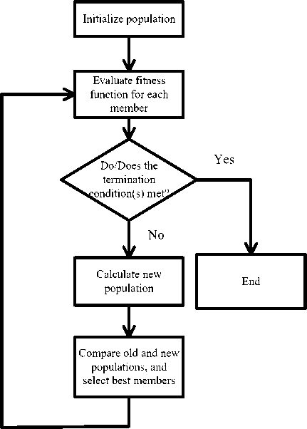
Fig. 1. Flow diagram of Differential Evolution Algorithm x4 0 = XjL + rand(xU-XjL) (4)

where x j L and x j U are upper and lower bound of the search space.

After the completion of the initialization phase, a new mutated population ( V ) is calculated from the initial population ( X ). This new population is formulated in (5).

V ik = h ., k , v» ‘ ,..., V i , Dk J (5)

In this study eight different mutation operators are used for comparison. The temporary V population is calculated by applying one of these eight mutation operators. The next subsection explains these mutation operators.

Following the mutation operator, the crossover is executed to new population U as given in (6).

U_t^k =\u_t ,1 ^k , u i ,2 k ,..., u i , D^k ^J ⁽⁶⁾

Table 1. Ten Multimodal Benchmark Problems

No	Name of Function	Mathematical Expression of Function		Domain
F 1	Five-Uneven-Peak Trap	F 1 ( x ) = •	‘ 80 ( 2.5 - x ) 0 < x < 2.5 64 ( x - 2.5 ) 2.5 < x < 5 64 ( 7.5 - x ) 5 < x < 7.5 28 ( x - 7.5 ) 7.5 < x < 12.5 28 ( 17.5 - x ) 12.5 < x < 17.5 32 ( x - 17.5 ) 17.5 < x < 22.5 32 ( 27.5 - x ) 22.5 < x < 27.5 80 ( x - 27.5 ) 27.5 < x < 30	x e [ 0,30 ]
F 2	Equal Maxima	F₂ ( x ) = sin⁶ ( 5 nx )		x e [ 0,1 ]
F 3	Uneven Decreasing Maxima	F ( x ) = exp [- 2log ( 2 ) [ ' ° J’ \| sin * ( 5 , Г x 34 - 0.05 )1 ³ ( ^v 1 0.854 J J v V JJ		x e [ 0,1 ]
F 4	Himmelblau	F 4 ⁽ x , y ) = ²⁰⁰ ^-( ^x ^{2 +} y - ll ) ^-( ^x ⁺ y 2 ^- 7 )		x e [ 0,1 ]
F 5	Six-Hump Camel Back	Г[ x 1 F 5 ( x , У ) = - 4 1 4 - 2.1 x + y J x + xy + ( 4 y - 4 ) y		x e [ - 1.9,1.9 ] y ^{e [-} ¹.^1,1.¹ ^]
F 6	Shubert 2D	55 F_e ( x , У ) = - ^ i cos [ ( i + 1 ) x + i ] ^ i cos [ ( i + 1 ) У + i ] i = 1 i = 1		x e [ - 10,10 ] У e [ - 10,10 ]
F 7	Vincent 2D	F ₇ ( x , y ) = ¹ ( sin ( 10log ( x )) + sin ( 10log ( y )))		x e [ 0.25,10 ] y e [ 0.25,10 ]
F 8	Shubert 3D	F , ( x ) = " П [] t i cos [ ( i + 1 ) x + i ] \| j = 1 V i = 1 J		x j e [ - 10,10 ]
F 9	Vincent 3D	F 9 ⁽ ^x ) = ¹ y t sin l lOlog l x i ))) ³ i = 1		x i e [ 0.25,10 ]
F 10	Modified Rastrigin	F ₀( x , y ) = - ( 10 + 9cos ( * nx )) - ( 10 + 9cos ( 8 ny ))		x e [ 0,1 ] У e [ 0,1 ]

Two fundamental crossover operators were defined for DE. However, from the researches [20-22] it is emphasize that none of them is superior each other. These crossover operators are exponential and binomial operators. In this paper, binomial operator is selected, because the computation burden of binomial operator is lower than exponential, and also the performance of these two methods are equal.

k ^u i , j

= s

k i,j

i , j

rand < CR

The mathematical expression for binomial operator is presented in (7). The CR is an algorithm parameter and the value of CR assign differently for different mutation operators.

The last operator is called the selection. In the selection phase two populations X and U are compared and the best members among these two population are survived to the next generator. The number of survived members is equal to NP .

B. Mutation Operators

In this study, eight different mutation operators with crowding DE are compared with respect to performance measurement functions. In the next subsection the crowding operator will be explained. All these operator are taken F and CR as algorithm parameters which have the value depended on the mutation operator.

1) DE/Rand/1(F=0.8, CR=0.9)(DE-R1)

First mutation operator is called as DE/Rand/1 [21]. The method begins with the selection of three random vectors r 1 , r 2 and r 3 . Three random vectors and the current member of the population form a new member. The operator is given in (8) and graphically demonstrate in Figure 2.

k +1 k k k I

V = X , ■ +/* X т —X, I i , j r 1, j r 2, j r 3, j

Table 3. Peak Ratio (Success Rate) of Various Differential Evolution Algorithms on Benchmark Problems (Level of Accuracy = 0.1)

No	DE-B1	DE-B2	DE-R1	DE-R2	DE-RB	DE-RS	T-DE	TS-DE
F 1	0.50 (0)	0.56 (0.14)	1 (1)	0.72 (0.50)	0.46 (0)	1 (1)	0.49 (0)	1 (1)
F 2	1 (1)	1 (1)	1 (1)	1 (1)	1 (1)	1 (1)	1 (1)	1 (1)
F 3	0.40 (0.40)	0.50 (0.50)	1 (1)	1 (1)	0.42 (0.42)	1 (1)	0 (0)	1 (1)
F 4	1 (1)	0.995 (0.98)	1 (1)	1 (1)	1 (1)	1 (1)	1 (1)	1 (1)
F 5	0.96 (0.92)	1 (1)	1 (1)	1 (1)	1 (1)	1 (1)	1 (1)	1 (1)
F 6	22E^-3(0)	31.1E^-3 (0)	0.30 (0)	18.9E^-3 (0)	32.2E^-3 (0)	23.3E^-3(0)	23.3E^-3(0)	23.3E^-3 (0)
F 7	92.2E^-3 (0)	55E^-3(0)	0 (0)	0 (0)	80E^-3(0)	0 (0)	1.1E^-3 (0)	1.1E^-3 (0)
F 8	0 (0)	0 (0)	0 (0)	0 (0)	0 (0)	0 (0)	0 (0)	0 (0)
F 9	3.61E^-3 (0)	2.2E^-3(0)	0 (0)	0 (0)	2.78E^-3 (0)	0 (0)	64.8E^-5(0)	64.8E^-5 (0)
F 10	72.7E^-2(0.28)	93.7E^-2 (0.82)	1 (1)	1 (1)	1 (1)	1 (1)	1 (1)	1 (1)

Table 4. Statistics for Number of Peaks of Various Differential Evolution Algorithms on Benchmark Problems (Level of Accuracy = 0.1)

No		DE-B1	DE-B2	DE-R1	DE-R2	DE-RB	DE-RS	T-DE	TS-DE
F 1	Max.	1	2	2	2	1	2	1	2
	Min.	1	0	2	0	0	2	0	2
	Mean	1	1,12	2	1.44	0.92	2	0.98	2
	Std.Dev	0	38.5E^-2	0	61.1E^-2	27.4E^-2	0	14.1E^-2	0
F 2	Max.	5	5	5	5	5	5	5	5
	Min.	5	5	5	5	5	5	5	5
	Mean	5	5	5	5	5	5	5	5
	Std.Dev	0	0	0	0	0	0	0	0
F 3	Max.	1	1	1	1	1	1	0	1
	Min.	0	0	1	1	0	1	0	1
	Mean	0.40	0.50	1	1	0.42	1	0	1
	Std.Dev	49.4E^-2	50.5E^-2	0	0	49.8E^-2	0	0	0
F 4	Max.	4	4	4	4	4	4	4	4
	Min.	4	3	4	4	4	4	4	4
	Mean	4	3.98	4	4	4	4	4	4
	Std.Dev	0	14.1E^-2	0	0	0	0	0	0
F 5	Max.	2	2	2	2	2	2	2	2
	Min.	1	2	2	2	2	2	2	2
	Mean	1.92	2	2	2	2	2	2	2
	Std.Dev	27.4E^-2	0	0	0	0	0	0	0
F 6	Max.	3	2	2	2	3	4	2	2
	Min.	0	0	0	0	0	0	0	0
	Mean	0.40	0.56	0.54	0.34	0.58	0.42	0.42	0.42
	Std.Dev	69.9E^-2	64.6E^-2	64.5E^-2	51.9E^-2	64.1E^-2	75.8E^-2	60.9E^-2	60.9E^-2
F 7	Max.	10	11	0	0	13	0	1	1
	Min.	0	0	0	0	0	0	0	0
	Mean	3.32	1.98	0	0	2.88	0	_4E-2	0.40
	Std.Dev	2.75	2.54	0	0	4.11	0	19.7E^-2	19.7E^-2
F 8	Max.	0	0	0	0	0	0	0	0
	Min.	0	0	0	0	0	0	0	0
	Mean	0	0	0	0	0	0	0	0
	Std.Dev	0	0	0	0	0	0	0	0
F 9	Max.	5	6	0	0	8	0	2	2
	Min.	0	0	0	0	0	0	0	0
	Mean	0.78	0.48	0	0	0.60	0	0.14	0.14
	Std.Dev	1.16	1.05	0	0	1.45	0	45.2E^-2	45.2E^-2
F 10	Max.	12	12	12	12	12	12	12	12
	Min.	3	4	12	12	12	12	12	12
	Mean	8.72	11.24	12	12	12	12	12	12
	Std.Dev	2.99	1.83	0	0	0	0	0	0

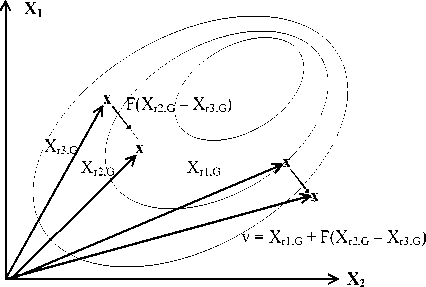
Fig. 2. Graphical demonstration of DE/Rand/1 Mutation Operator.

population. The formulation increases the convergence speed of the algorithm. As the iteration approach to the maximum iteration value, the optima are began to search around the best solution. This increases the convergence, however, still local optimum problem couldn't able to solve with this mutation algorithm.

Figure 2 gives the graphical demonstration of DE/Rand/1 mutation operator. Randomly three solution candidates are selected from population. Scaled difference between two randomly selected solution is added to other randomly selected solution. As the solutions are converges to the global/local optima, the difference between any two randomly selected solution becomes smaller. Hence, at the beginning of each iteration, the algorithm can search larger areas of search space (as seen in Figure 2). However, if the algorithm converges to local optima, the mutation operator couldn't help the algorithm to escape from local optima.

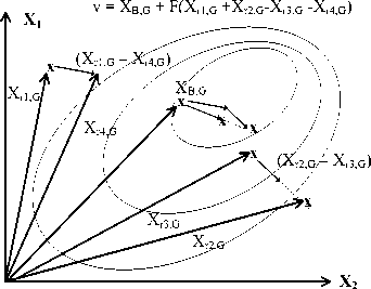
2) DE/Best/1(F=0.8, CR=0.9)(DE-B1)

This operator depends on the best member in the population [21]. Similarly, this best member is used instead of first random vector in DE/Rand/1. The formulation of the operator is given in (9) and graphically demonstrated in Figure 3.

k + 1 k k k

v i , j = x B , j ⁺ ^F ( x r 2, j x r 3, j ) (9)

Figure 3 gives graphical demonstration for DE/Best/1. The only difference is instead of three randomly selected solution candidates, only two solutions are selected randomly and the best particle is added to the formulation. the best particle means that, the solution candidate present the smallest (for minimization problem and largest for maximization problems) cost value inside the

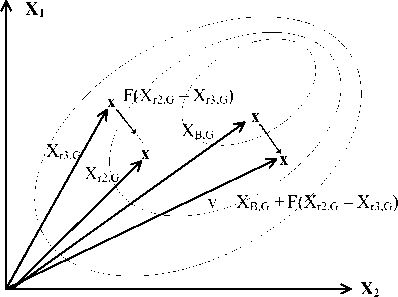
Fig. 3. Graphical demonstration of DE/Best/1 Mutation Operator.

3) DE/Rand-to-Best/1(F=0.8, CR=0.9, λ=0.8) (DE-RB)

This method is the joint implementation of DE/Rand-1 and DE/Best/1 [21]. Instead of direct use of randomly selected vectors, the difference between vectors is calculated. The general form of this operator is presented in (10).

k + 1 k k k k k

vuj = x.,j + ДXB,j - xi,j )+ F(xr2,j - xr3,j ) (10)

In (10), one more algorithm parameter is added. This parameters increases the complexity of the algorithm since one more parameter needs be settled. Hence, to reduce the complexity of the method λ = F is selected. Therefore the final form of the method is presented in (11), and demonstrated in Figure 4.

k + 1 k k k k k

vi,j = xi,j + F(xr2,j - xr3,j + xB,j - xi,j ) (11)

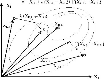
Fig. 4. Graphical demonstration of DE/Rand-to-Best/1 Mutation Operator.

Figure 4 shows the collaboration of previous DE mutation algorithms. The aim is to increase the search and convergence ability of DE. The scale difference between two randomly selected solution and scaled difference between best solution and the current position is added as step to the current solution. The three terms are added to form a new mutated solution. First term is the starting point, second term is for improvement of convergence and the last term is for increasing the search capability. This formulation is very similar to Particle Swarm Optimization velocity update rule.

4) DE/Best/2(F=0.8, CR=0.9)(DE-B2)

This method considers four randomly determined vectors r 1 , r 2 , r 3 and r 4 [21].

Table 5. Peak Ratio (Success Rate) of Various Differential Evolution Algorithms on Benchmark Problems

ε = 0.01 ε = 0.001 No DE-R1 DE-RS TS-DE DE-R1 DE-RS TS-DE F1 0.33 (0.12) 0.34 (0.18) 0.85 (0.7) 0.05 (0) 0.07 (0) 0,25 (0.02) F2 1 (1) 1 (1) 1 (1) 1 (1) 1 (1) 1 (1) F3 0.96 (0.96) 0.98 (0.98) 0.96 (0.96) 0.92 (0.92) 0.94 (0.94) 0.96 (0.96) F4 1 (1) 1 (1) 1 (1) 64.5E-2 (0.18) 81.5E-2(0.52) 1 (1) F5 1 (1) 1 (1) 1 (1) 1 (1) 1 (1) 1 (1) F6 1.1E-3 (0) 3.3E-3 (0) 4.4E-3(0) 0 (0) 0 (0) 0 (0) F10 1 (1) 1 (1) 99.1E-3(0.98) 46.7E-2 (0.02) 0.43 (0.02) 53.1E-2 (0.1) k+1 - x k k-x k k-x kkl3)

v i , j = x r 1, j ⁺ F 1 \ x r 2, j x r 3, j + F 2 x r 4, j x r 5, j / ^{( J)}

k+1 k k k k k vi,j = xB,j + F(xr 1,j + xr2,.j - xr3,.j - xr4,.j ) (12)

k +1 k k k k k i, j r1, j r4, j r5, j r2,j r3,j

Fig. 5. Graphical demonstration of DE/Best/2 Mutation Operator

Figure 5 is the good example for explaining DE/Best/2 mutation method. As the result obtained in Fig. 5 is revealed that the aim is to increase the convergence. however, at the beginning of iteration, the solution is search on a circle (for 2D problem) around best solution. Hence, the fast convergence ban be obtain by this formulation, however, also the algorithm can be seem highly fall into the local optima.

5) DE/Rand/2(F1=0.8, F2=0.8, CR=0.9)(DE-R2)

Five randomly determined vectors with two algorithm parameters are needed for this method. Similar to DE/Rand-toBest/1 method, these two algorithm parameters are selected as equal, as given in (13) and (14) respectively [21]. The mutation operator given in (13) graphically demonstrated in Figure 6.

The idea of mutation operator given in Fig. 6 is very similar to Fig. 5. The mail difference is that the search capability of DE/Rand/2 is better than DE/Best/2 since instead of best particle, the solution is searched on a randomly selected solution. It means that to decrease the convergence speed gives result to search larger areas. That reduces the problem of local optima.

6) Trigonometric Mutation (F=0.5,CR=0.9, Γ=0.05) (T-

DE)

The aim of this method is to increase convergence property of DE [23]. Similarly, this method depends of three randomly selected vectors ( r ₁, r ₂, r ₃). By using the fitness values of thee randomly selected vectors, three more parameters are calculated, which are presented in (15) to (18).

P' =| f (Xr 1, G )+| f (Xr 2,G ) + | f (Xr 3,G )

Px =|f (Xr 1,G ) / P'

P2 =|f (Xr2,G ) / P'

P3 =|f (Xr3,G ) / P'

The trigonometric mutation operator is calculated by using three new parameters. The final formulation of the operator is given in (19), where Γ is the new algorithm parameter.

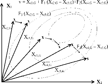
Fig. 6. Graphical demonstration of DE/Rand/2 Mutation Operator

'( X r 1, G + X ,

r 2, G ⁺ ^Xr 3, G )

k + 1

= <

⁽ ^P 2 - ^P 1 ⁾⁽ ^Xr 1, G - ^Xr 2, G ⁾ ⁺ ⁽ ^P 3 - ^P 2 ⁾⁽ ^Xr 2, G - ^Xr 3, G ⁾ ⁺

⁽ ^P 1 ^P 3 ⁾⁽ ^Xr 3, G ^Xr 1, G )

rand < Г

^Xr 1 ⁺ ^F ⁽ ^Xr 2, G ⁺ ^Xr 3, G ) otherwise

Table 6. Statistics for Number of Peaks of Various Differential Evolution Algorithms on Benchmark Problems

		ε = 0.01			ε = 0.001
No		DE-R1	DE-RS	TS-DE	DE-R1	DE-RS	TS-DE
F 1	Max.	2	2	2	1	1	2
	Min.	0	0	1	0	0	0
	Mean	0.66	0.68	1.7	0.10	0.14	0.50
	Std.Dev	68.8E^-2	76.7E^-2	46.2E^-2	30.3E^-2	35.1E^-2	54.3E^-2
F 2	Max.	5	5	5	5	5	5
	Min.	5	5	5	5	5	5
	Mean	5	5	5	5	5	5
	Std.Dev	0	0	0	0	0	0
F 3	Max.	1	1	1	1	1	1
	Min.	0	0	0	0	0	0
	Mean	0.96	0.98	0.96	0.92	0.94	0.96
	Std.Dev	19.7E^-2	14.1E^-2	19.7E^-2	27.4E^-2	23.9E^-2	19.7E^-2
F 4	Max.	4	4	4	4	4	4
	Min.	4	4	4	0	1	4
	Mean	4	4	4	2.58	3.26	4
	Std.Dev	0	0	0	1.01	89.9E^-2	0
F 5	Max.	2	2	2	2	2	2
	Min.	2	2	2	2	2	2
	Mean	2	2	2	2	2	2
	Std.Dev	0	0	0	0	0	0
F 6	Max.	1	1	2	0	0	0
	Min.	0	0	0	0	0	0
	Mean	0.02	0.06	0.08	0	0	0
	Std.Dev	14.1E^-2	23.9E^-2	34.1E^-2	0	0	0
F 10	Max.	12	12	12	12	12	12
	Min.	12	12	7	0	0	0
	Mean	12	12	11.9	5.60	5.16	6.38
	Std.Dev	0	0	70.7E^-2	2.69	2.91	3.32

7) Random Scale Mutation (DE-RS) and Time Varying Scale Mutation(TS-DE) (Fmax=1, Fmin=0, CR=0.9) Two other mutation operators which are related to determination of the algorithm parameter of F are considered in this paper [24]. These operators are used with DE/Rand/1 mutation scheme. The parameter assignments are defined in (20) and (21) respectively.

F (i ) = 0.5 ( 1 + rand (0,1) ) (20)

F ⁽ i ) = ⁽ ^F max - ^F min X. max iter - i ) ⁽²¹⁾

C. Crowding

Crowding is based on the natural phenomenon such that in nature since there are limited number of fundamental resources to survive, living beings have to compete each similar members for limited resources. Therefore members of the same family of animals finds the proper living environment and adopts the conditions of this new environment (behavior adaptation). One of the fundamental reason to form groups of animals is the distance or more simple the ability to reach the resources.

In a similar manner, crowding scheme is based on the distance between solution candidates. The cost value of an offspring (in evolutionary computing) is compared with the cost value of the nearest individual (Euclidean distance is preferred for measuring the distance) in the current population. The number of solution candidates which are selected for replacement is determined by the constant parameter called crowding factor (CF). For improper selected CF values, a problem called replacement error may emerge. This problem is caused by the replacing of non similar members. Even this problem can affect the solution quality of the algorithm, the solution is very simple that setting CF equal to the number of individuals in the population as proposed in [9]. Crowding scheme has a basic layout especially for evolutionary algorithms. In case of DE, the last phase (selection) of DE is change from the selection to the crowding. The crowding method is summarized as

a) calculate Euc ( x i , u i ), which is Euclidean distance between X and U ,
b) find the member of X which has the minimum Euclidean distance to u _i,
c) if fitness value of u _i is smaller than x_i then replace.

III. Implementation Results

Eight different mutation operators of DE are evaluated on ten benchmark problems with 600 iterations, 100 number of members, 50 independent run, and performance of variations are compared with respect to performance measurement functions. The implementation are compared as a competition based on different levels of accuracy, which is a threshold level under which is consider a global optimum is found ( ε =0.1; ε =0.01; ε =0.001; ε =0.0001).

A. Benchmark Problems

The benchmark problems are previously well defined functions which have different multiple optima [25]. The importance of benchmark problems are

a) the number of multiple optima and
b) their position and fitness values are known
c) it is easy to compare other studies with the well-known problems.

Table 1 presents multimodal benchmark problems, and Table 2 gives the number of global optima of the benchmark functions.

B. Performance Measurement

The performance of algorithms is measured by using two criteria, which are called peak ratio ( PR ) and success rate ( SR ). The PR and SR are performance measure variables defined in [0,1]. The PR is the proportion of total number of global optima found in the end of each run to the total number of global optima. The (22) explains PR as mathematical formula.

NR у NPF run

PR = run = 1 (22)

NKP x NR where NPFrun is the number of global optima found in the end of ith run, NKP is the number of known global optima, and NR is the number of run.

The SR is a more general/overall sign for performance. SR gives the number of successful run against all run as given in (23).

NSR

SR =---

Table 2. Parameters for Benchmark Problems

Function Name Niche Radius Number of Global Optima F1 0.01 2 F2 0.01 5 F3 0.01 1 F4 0.01 4 F5 0.5 2 F6 0.5 18 F7 0.2 36 F8 0.5 81 F9 0.2 216 F10 0.01 12 where NSR is the number of successful runs that all of the global optima is detected by algorithm. These performance measurement variables depend on the location of global optima. Hence first it must be determined such that global optima is close enough within accuracy level (ε), and the solution is within the niche radius from all global solutions. Table 2 gives niche radius and number of global optima for each benchmark problems.

C. Results

There are eight different algorithms, ten benchmark problems and two performance measurement techniques are applied on four accuracy levels. Since the accuracy levels represent the degree of difficulty, competition based implementations are executed. Therefore four sets of implementation are defined for each level of accuracy. After each implementation set, some algorithms and benchmark problems are executed from comparison list based on the performance of algorithms on problems.

First, for ε =0.1 level of accuracy, eight algorithms are evaluated, and Table 3 presents PR and SR performance measures of these algorithms for ten benchmark functions. Table 3 shows that for functions F 7 - F 9 all algorithms cannot able to locate any global optima due to the success rates for these problems are zero. The performance of DE-R1, DE-RS, and TS-DE have the best among all algorithms.

Table 4 gives the statistical data about number of found optima (number of peaks). These data contain minimum, maximum, mean and standard deviation of the number of obtain global optima. The algorithms DE-R1, DE-RS, TS-DE can able to find all peak points for a given level of accuracy at problems F 1 - F 5 and F 12 . The benchmark problems with a high number of peaks ( F 6 - F 9 ), which are hardest problems, cannot be solved by and of eight algorithms. But for the functions F ₆, F ₇ and F ₉, the algorithms can able to find some of peaks. Therefore, from first implementation set only three algorithms and six benchmark problems can able to survive to the next competition since the performance of other methods fall behind. The algorithms which can be able to reach to the next competition are DE/Rand/1, Random Scale and Time varying scale, and the problems are F ₁- F ₅ and F ₁₀.

Second and third set of implementations for ε =0.01 and ε =0.001 are evaluated for comparing three algorithms on six benchmark problems, and results presented in Table 5 and Table 6, respectively. Table 5 gives peak ratio and success rate of algorithms. It isn't possible to present a general conclusion about algorithm since for ε =0.01 and for functions F 2 , F 4 - F 5 , the algorithms result are same performance, but for other functions TS-DE outperforms for other algorithms. For ε =0.001, for functions F ₂, F ₅- F ₆, the algorithms result are same performance, but similarly TS-DE outperforms for other functions.

Table 6 gives statistics for number of peaks that are found by algorithms. Table 6 presented for two levels of accuracy ε=0.01 and ε=0.001. The results in Table 6 also supports the results of Table 5, such that even all algorithms are presented almost same performance, TS-DE slightly presents better performance when compared with other algorithms. From the evaluations of all results given in Table 5 and 6, it is seen that the results are similar to each other, for a better conclusion, another implementation is executed for last level of accuracy.

Table 7. Results for Benchmark Problems

No		DE-R1	DE-RS	TS-DE
F 1	Max.	1	0	1
	Min.	0	0	0
	Mean	0.02	0	0.06
	Std.Dev	14.1E^-2	0	23.9E^-2
	SR	0	0	0
	PR	0.01	0	0.03
F 2	Max.	5	5	5
	Min.	5	5	5
	Mean	5	5	5
	Std.Dev	0	0	0
	SR	1	1	1
	PR	1	1	1
F 3	Max.	1	1	1
	Min.	0	0	0
	Mean	0.54	0.68	0.96
	Std.Dev	50.3E^-2	47.1E^-2	19.7E^-2
	SR	0.45	0.68	0.96
	PR	0.54	0.68	0.96
F 4	Max.	2	2	4
	Min.	0	0	3
	Mean	0.48	0.60	3.9
	Std.Dev	61.4E^-2	60.6E^-2	30.3E^-2
	SR	0	0	0.9
	PR	0.12	0.15	0.975
F 5	Max.	5	5	5
	Min.	5	5	5
	Mean	5	5	5
	Std.Dev	0	0	0
	SR	1	1	1
	PR	1	1	1
F 10	Max.	2	4	5
	Min.	0	0	0
	Mean	0.44	0.84	1.14
	Std.Dev	61.1E^-2	1.05	1.38
	SR	0	0	0
	PR	0.03	0.07	9.5E^-2

The last implantation is made for level of accuracy ε =0.0001. Three algorithms are compared on six benchmark problems and performance of these algorithms are presented in Table 7. For functions F 2 and F ₅, the performance of all algorithms are the same each other. However, when considered other benchmark problems, TS-DE outperforms when compared with others. In summary, from the Tables 3-7, the performance of different algorithms show that time varying DE outperforms against other DE algorithms.

IV. Conclusion

This study compares eight different DE variants for ten multimodal benchmark problems. The aim of this paper is to propose a reliable crowding DE algorithm for multimodal problems. From the results, it can be concluded that as the number of global optima increases the performance of crowding DE decreasing for all variants. It isn't possible to obtain good results for benchmark problems after 18 global optimums for crowding DE algorithms, and from eight variants, only time varying crowding DE performs better for all level of accuracy. From literature review, it was seen that DE-R1 and DE-B1 algorithms are used as crowding DE. From the results obtained in this study showed that, DE-B1 couldn't able to survive for the last implementation set. Also, even DE-R1 reaches to the last comparisons, the performance of DE-R1 is lower than TS-DE. From the point of execution times of DE-R1, DE-B1 and TS-DE, DE-B1 is the slowest algorithm since the mutation operator needs to find best member in the population. Since TS-DE is the improved version of DE-R1, DE-R1 has the fastest execution mutation code. But, the code difference between DE-R1 and TS-DE is only a line of mathematical operation contains a difference and a multiplication, which adds relatively small amount of time to the commutative execution time.

Acknowledgment

This study is made possible by a grant from TUBITAK 2214/A Research Scholar Program for PhD Students. The author would like to express his gratitude for their support.

Список литературы A Comparison of Crowding Differential Evolution Algorithms for Multimodal Optimization Problems

B.Y. Qu, P.N. Suganthan, S. Das, “A distance-based locally informed particle swarm model for multimodal optimization,” IEEE Transactions on Evolutionary Computation, vol. 17, no. 3, pp. 387-402, 2013.
S.W. Mahfoud, Niching methods for genetic algorithms. PhD Thesis, Department of Computer Sciences, University of Illinois Urbana-Champaign, 1995.
N.N. Glibovets, N.M. Gulayeva, “A review of niching genetic algorithms for multimodal function optimization,” Cybernetics and Systems Analysis, vol. 49, no. 6, pp. 815-820, 2013.
X. Zhang, L. Wang, B. Huang, “An improved niche ant colony algorithm for multi-modal function optimization,” International Conference on Instrumentation & Measurement Sensor Network and Automation, pp. 403-406, 2012.
B.Y. Qu, J.J. Liang, P.N. Suganthan, “Niching particle swarm optimization with local search for multi-modal optimization,” Information Sciences, vol. 197, pp. 131-143, 2012.
S.C. Esquivel, C. Coello Coello, “On the use of particle swarm optimization with multimodal functions,” The Congress on Evolutionary Computation, pp. 1130-1136, 2003.
L. Yu, X. Ling, Y. Liang, M. lv, G. Liu, “Artificial bee colony algorithm for multimodal function optimization,” Advances Science Letters, vol. 11, no. 1, pp. 503-506, 2012.
S. Biswas, S. Kundu, S. Das, “Inducing niching behavior in differential evolution through local information sharing,” IEEE Transactions on Evolutionary Computation, Early Access.
R. Thomsen, “Multimodal optimization using crowding-based differential evolution,” The Congress on Evolutionary Computation, pp. 1382-1389, 2004.
D. Shen, Y. Li, “Multimodal optimization using crowding differential evolution with spatially neighbors best search,” Journal of Software, vol. 8, no. 4, pp. 932-938, 2013.
B. Sareni, L. Krahenbuhl, “Fitness sharing and niching methods revisited,” IEEE Transactions on Evolutionary Computation, vol.2, no. 3, pp. 1382-1389, 2004.
O. Mengsheal, D. Goldberg, “Probabilistic crowding, deterministic crowding with probabilistic replacement,” GECCO, pp. 409-416, 1999.
J.E. Vitela, o. Castona, “A real-coded niching memetic algorithm for continuous multimodal function optimization,” The Congress on Evolutionary Computation, pp. 2170-2177, 2008.
D. Cavicchio, Adapting search using simulated evolution. PhD Thesis, Department of Industrial Engineering, University of Michigan Ann Arbor, 1970.
B.L. Miller, M.J. Shaw, “Genetic algorithms with dynamic niche sharing for multimodal function optimization,” International Conference on Evolutionary Computation, pp. 786-791, 1996.
D.E. Goldberg, J. Richardson, “Genetic algorithms with sharing for multimodal function optimization,” International Conference on Genetic Algorithms, pp. 41-49, 1987.
L. Qing, W. Gang, Y. Zaiyve, W. Qiuping, “Crowding clustering genetic algorithm for multimodal function optimization,” Applied Soft Computing, vol. 8, no. 1, pp. 88-95, 2008.
S. Kamyab, M. Eftekhari, “Using a self-adaptive neighborhood scheme with crowding replacement memory in genetic algorithm for multimodal optimization,” Swarm and Evolutionary Computation, vol. 12, pp. 1-17, 2013.
R. Storn, K. Price, Differential evolution - a simple and efficient adaptive scheme for global optimization over continuous space. International Computer Science Institute, Technical Report, TR-95-012, 1995.
R. Storn, Differential evolution design of an IIR-filter with requirements for magnitude and group delay. International Computer Science Institute, Technical Report, TR-95-026, 1995.
R. Storn, “Differential evolution design of an IIR-filter with requirements for magnitude and group delay,” International Conference on Evolutionary Computation, pp. 268-273, 1995.
R. Storn, “On the usage of differential evolution for function optimization,” North America Fuzzy Information Processing Society, pp. 519-523, 1996.
H.Y. Fan, J. Lampinen, “A trigonometric mutation operation to differential evolution,” Journal of Global Optimization, vol. 27, no. 1, pp. 105-129, 2003.
S. Das, A. Konar, U.K. Chakrabarty, “Two improved differential evolution schemes for faster global search,” GECCO, pp. 991-998, 2005.
X. Li, A. Engelbrecht, M.G. Epitropakis, Benchmark function for CEC2013 Special Session and competition on niching methods for multimodal function optimization. Technical Report, Evolutionary Computation and Machine Learning Group, RMIT University, Australia, 2012.

Еще

Статья научная